pacman::p_load(sf, tidyverse, tmap, tidyverse, corrplot, funModeling, corrplot, psych, ggpubr, cluster, factoextra, heatmaply, spdep, ClustGeo, rgdal, NbClust, GGally, patchwork, ggthemes, knitr)Take-home EX2
Take-home Exercise 2: Regionalisation of Multivariate Water Point Attributes with Non-spatially Constrained and Spatially Constrained Clustering Methods
Setting the Scene
The process of creating regions is called regionalisation. A regionalisation is a special kind of clustering where the objective is to group observations which are similar in their statistical attributes, but also in their spatial location. In this sense, regionalization embeds the same logic as standard clustering techniques, but also applies a series of geographical constraints. Often, these constraints relate to connectivity: two candidates can only be grouped together in the same region if there exists a path from one member to another member that never leaves the region. These paths often model the spatial relationships in the data, such as contiguity or proximity. However, connectivity does not always need to hold for all regions, and in certain contexts it makes sense to relax connectivity or to impose different types of geographic constraints.
Objectives
In this take-home exercise you are required to regionalise Nigeria by using, but not limited to the following measures:
Total number of functional water points
Total number of nonfunctional water points
Percentage of functional water points
Percentage of non-functional water points
Percentage of main water point technology (i.e. Hand Pump)
Percentage of usage capacity (i.e. < 1000, >=1000)
Percentage of rural water points
The Data
Apstial data
For the purpose of this assignment, data from WPdx Global Data Repositories will be used. There are two versions of the data. They are: WPdx-Basic and WPdx+. You are required to use WPdx+ data set.
Geospatial data
Nigeria Level-2 Administrative Boundary (also known as Local Government Area) polygon features GIS data will be used in this take-home exercise. The data can be downloaded either from The Humanitarian Data Exchange portal or geoBoundaries.
The Task
The specific tasks of this take-home exercise are as follows:
Using appropriate sf method, import the shapefile into R and save it in a simple feature data frame format. Note that there are three Projected Coordinate Systems of Nigeria, they are: EPSG: 26391, 26392, and 26303. You can use any one of them.
Using appropriate tidyr and dplyr methods, derive the proportion of functional and non-functional water point at LGA level (i.e. ADM2).
Combining the geospatial and aspatial data frame into simple feature data frame.
Delineating water point measures functional regions by using conventional hierarchical clustering.
Delineating water point measures functional regions by using spatially constrained clustering algorithms.
Thematic Mapping
- Plot to show the water points measures derived by using appropriate statistical graphics and choropleth mapping technique.
Analytical Mapping
- Plot functional regions delineated by using both non-spatially constrained and spatially constrained clustering algorithms.
Glimpse of Steps
Some of the important steps performed in this study are as follows
Importing shapefile into R using sf package.
Deriving the proportion of functional and non-functional water point at LGA level using appropriate tidyr and dplyr methods.
Combining the geospatial and aspatial data frame into simple feature data frame.
Delineating water point measures functional regions by using conventional hierarchical clustering.
Delineating water point measures functional regions by using spatially constrained clustering algorithms.
Thematic Mapping - Plotting maps to show the water points measures derived by using appropriate statistical graphics and choropleth mapping technique.
Analytical Mapping - Plotting functional regions delineated by using both non-spatially constrained and spatially constrained clustering algorithms.
Loading packages
Let us first load required packages into R environment. p_load function pf pacman package is used to install the following packages into R environment.
sf, rgdal and spdep - Spatial data handling
tidyverse, especially readr, ggplot2 and dplyr - Attribute data handling
tmap - Choropleth mapping
coorplot, ggpubr, and heatmaply - Multivariate data visualisation and analysis
cluster, ClustGeo - Cluster analysis
patchwork, ggthemes - Effective visualisation and layouts
Importing Spatial Data
Import spatial data. Since water point data set is in csv file format, we will use read_csv() of readr package to import WPdx.csv as shown the code chunk below. The output R object is called listings and it is a tibble data frame.
filter()of dplyr package is used to extract water point records of Nigeria.
wp_nga <- read_csv("data/WPdx.csv") %>%
  filter(`#clean_country_name` == "Nigeria")
st_as_sfc() of sf package is used to derive a new field called Geometry as shown in the code chunk below
wp_nga$Geometry = st_as_sfc(wp_nga$`New Georeferenced Column`)convert the tibble data frame into sf data frame.
wp_sf <- st_sf(wp_nga, crs=4326) Importing Geospatial Data
Now let us import geospatial data. The code chunk below uses st_read() function of sf package to import geoBoundaries-NGA-ADM2 shapefile into R environment.
Two arguments are used :
dsn - destination : to define the data path
layer - to provide the shapefile name
crs - coordinate reference system in epsg format. EPSG: 4326 is wgs84 Geographic Coordinate System
nga <- st_read(dsn = "data",
               layer = "geoBoundaries-NGA-ADM2",
               crs = 4326) %>%
  select(shapeName)
Reading layer `geoBoundaries-NGA-ADM2' from data source `C:\HzzZZ11\ISSS624\Take-home_EX\Take-home Ex2\data' using driver `ESRI Shapefile' Simple feature collection with 774 features and 5 fields Geometry type: MULTIPOLYGON Dimension: XY Bounding box: xmin: 2.668534 ymin: 4.273007 xmax: 14.67882 ymax: 13.89442 Geodetic CRS: WGS 84Checking duplicate area name
duplicated can retrieve which elements of a vector or data frame are duplicate. The code chunk below can be used to determine the duplicate elements.
nga <- (nga[order(nga$shapeName), ])
nga<- nga %>%
mutate(shapeName = tolower(shapeName))
duplicate_Name <- nga$shapeName[ nga$shapeName %in% nga$shapeName[duplicated(nga$shapeName)] ]

duplicate_Name
[1] "bassa" "bassa" "ifelodun" "ifelodun" "irepodun" "irepodun"
[7] "nasarawa" "nasarawa" "obi" "obi" "surulere" "surulere"There are 12 duplicate elements. The below chunk assigns the right shape names corresponding to index values
nga$shapeName[c(94,95,304,305,355,356,518,519,546,547,693,694)] <- c("Bassa (Kogi)","Bassa (Plateau)",
                                                                               "Ifelodun (Kwara)","Ifelodun (Osun)",
                                                                               "Irepodun (Kwara)","Irepodun (Osun)",
                                                                               "Nassarawa (Kano)","Nassarawa",
                                                                               "Obi (Benue)","Obi(Nasarawa)",
                                                                               "Surulere (Lagos)","Surulere (Oyo)")

length((nga$shapeName[ nga$shapeName %in% nga$shapeName[duplicated(nga$shapeName)] ]))
[1] 0No duplicate values since the output is 0.
Combining geospatial and aspatial data
Transfer the attribute information in nga sf data frame into wp_sf data frame using st_join()function.
wp_sf <- st_join(wp_sf, nga)Renaming the column names
Rename some of the column names which begins with # for ease of use by using rename() function
wp_sfT <- wp_sf %>%
  rename ("Country" = "#clean_country_name",
          "clean_adm2" = "#clean_adm2",
          "status" = "#status_clean",
          "lat" = "#lat_deg",
          "long" = "#lon_deg",
          "water_tech" = "#water_tech_category") %>%
  mutate(status = replace_na(status, "Unknown"), water_tech = replace_na(water_tech, "Unknown")) %>%
  select (water_tech,clean_adm2,status,lat,long,usage_capacity, is_urban)
Extracting Funtional, Non-Functional and Unknown water points
Extract water point records by using #status_clean column.
functional <- wp_sfT %>%
  filter(`status` %in%  c("Functional", "Functional but not in use" , "Functional but needs repair")) %>%
  select(`lat`, `long`, `water_tech`, `clean_adm2`, `status`, `usage_capacity`, `is_urban`)

nonfunctional <- wp_sfT %>%
  filter(`status` %in%  c("Abandoned/Decommissioned", "Abandoned", "Non functional due to dry season", "Non-Functional", "Non-Functional due to dry season")) %>%
  select(`lat`, `long`, `water_tech`, `clean_adm2`, `status`, `usage_capacity`, `is_urban`)

unknown_wp <- wp_sfT %>%
  filter(`status` %in%  c("Unknown")) %>%
  select(`lat`, `long`, `water_tech`, `clean_adm2`, `status`, `usage_capacity`, `is_urban`)

handpump_count <- wp_sfT %>%
  filter(`water_tech` %in%  c("Hand Pump")) %>%
  select(`lat`, `long`, `water_tech`, `clean_adm2`, `status`, `usage_capacity`, `is_urban`)

usageL1k <- wp_sfT %>%
  filter(`usage_capacity` < 1000) %>%
  select(`lat`, `long`, `water_tech`, `clean_adm2`, `status`, `usage_capacity`, `is_urban`)

usage1k <- wp_sfT %>%
  filter(`usage_capacity` == 1000) %>%
  select(`lat`, `long`, `water_tech`, `clean_adm2`, `status`, `usage_capacity`, `is_urban`)

ruralWP <- wp_sfT %>%
  filter(`is_urban` == "FALSE") %>%
select(`lat`, `long`, `water_tech`, `clean_adm2`, `status`, `usage_capacity`, `is_urban`)st_crs(nga)Coordinate Reference System:
User input: EPSG:4326
wkt:
GEOGCRS["WGS 84",
ENSEMBLE["World Geodetic System 1984 ensemble",
MEMBER["World Geodetic System 1984 (Transit)"],
MEMBER["World Geodetic System 1984 (G730)"],
MEMBER["World Geodetic System 1984 (G873)"],
MEMBER["World Geodetic System 1984 (G1150)"],
MEMBER["World Geodetic System 1984 (G1674)"],
MEMBER["World Geodetic System 1984 (G1762)"],
MEMBER["World Geodetic System 1984 (G2139)"],
ELLIPSOID["WGS 84",6378137,298.257223563,
LENGTHUNIT["metre",1]],
ENSEMBLEACCURACY[2.0]],
PRIMEM["Greenwich",0,
ANGLEUNIT["degree",0.0174532925199433]],
CS[ellipsoidal,2],
AXIS["geodetic latitude (Lat)",north,
ORDER[1],
ANGLEUNIT["degree",0.0174532925199433]],
AXIS["geodetic longitude (Lon)",east,
ORDER[2],
ANGLEUNIT["degree",0.0174532925199433]],
USAGE[
SCOPE["Horizontal component of 3D system."],
AREA["World."],
BBOX[-90,-180,90,180]],
ID["EPSG",4326]]st_crs(wp_sfT)Coordinate Reference System:
User input: EPSG:4326
wkt:
GEOGCRS["WGS 84",
ENSEMBLE["World Geodetic System 1984 ensemble",
MEMBER["World Geodetic System 1984 (Transit)"],
MEMBER["World Geodetic System 1984 (G730)"],
MEMBER["World Geodetic System 1984 (G873)"],
MEMBER["World Geodetic System 1984 (G1150)"],
MEMBER["World Geodetic System 1984 (G1674)"],
MEMBER["World Geodetic System 1984 (G1762)"],
MEMBER["World Geodetic System 1984 (G2139)"],
ELLIPSOID["WGS 84",6378137,298.257223563,
LENGTHUNIT["metre",1]],
ENSEMBLEACCURACY[2.0]],
PRIMEM["Greenwich",0,
ANGLEUNIT["degree",0.0174532925199433]],
CS[ellipsoidal,2],
AXIS["geodetic latitude (Lat)",north,
ORDER[1],
ANGLEUNIT["degree",0.0174532925199433]],
AXIS["geodetic longitude (Lon)",east,
ORDER[2],
ANGLEUNIT["degree",0.0174532925199433]],
USAGE[
SCOPE["Horizontal component of 3D system."],
AREA["World."],
BBOX[-90,-180,90,180]],
ID["EPSG",4326]]Below code chunks create new columns of total water point count, functional/non-functional, unknown water points count, high/low usage water point count and water point count in non-urban region by using st_intersects() function.
nga$WPCount <- lengths(st_intersects(nga, wp_sfT))

nga$functional <- lengths(st_intersects(nga, functional))

nga$nonfunctional <- lengths(st_intersects(nga, unknown_wp))

nga$unknown_wp <- lengths(st_intersects(nga, nonfunctional))

nga$handpump <- lengths(st_intersects(nga, handpump_count))

nga$usage1k <- lengths(st_intersects(nga, usage1k))

nga$usageL1k <- lengths(st_intersects(nga, usageL1k))

nga$ruralWP <- lengths(st_intersects(nga, ruralWP))
Also the ratios of functional/non-functional, unknown water points, high/low usage water point and water point in non-urban region are been created.
nga <- nga %>%
  mutate(`pct_functional` = `functional`/`WPCount`) %>%
  mutate(`pct_nonfunctional` = `nonfunctional`/`WPCount`) %>%
  mutate(`pct_handpump` = `handpump`/`WPCount`) %>%
  mutate(`pct_usage1k` = `usage1k`/`WPCount`) %>%
  mutate(`pct_usageL1k` = `usageL1k`/`WPCount`) %>%
  mutate(`pct_ruralWP` = `ruralWP`/`WPCount`)
Removing NA values
nga <- nga[-c(3, 86, 241, 250, 252, 261, 400, 406, 447, 473, 492, 507, 526),]Replacing NA values
nga$`pct_functional`[is.na(nga$`pct_functional`)] <- 0
nga$`pct_nonfunctional`[is.na(nga$`pct_nonfunctional`)] <- 0
nga$`pct_handpump`[is.na(nga$`pct_handpump`)] <- 0
nga$`pct_usage1k`[is.na(nga$`pct_usage1k`)] <- 0
nga$`pct_usageL1k`[is.na(nga$`pct_usageL1k`)] <- 0
nga$`pct_ruralWP`[is.na(nga$`pct_ruralWP`)] <- 0
Transform the coordinates from 4326 to 26391 projection using the st_transform() function.
nga_sf <- st_transform(nga, crs = 26391)
st_crs(nga_sf)
Coordinate Reference System:
User input: EPSG:26391
wkt:
PROJCRS["Minna / Nigeria West Belt",
BASEGEOGCRS["Minna",
DATUM["Minna",
ELLIPSOID["Clarke 1880 (RGS)",6378249.145,293.465,
LENGTHUNIT["metre",1]]],
PRIMEM["Greenwich",0,
ANGLEUNIT["degree",0.0174532925199433]],
ID["EPSG",4263]],
CONVERSION["Nigeria West Belt",
METHOD["Transverse Mercator",
ID["EPSG",9807]],
PARAMETER["Latitude of natural origin",4,
ANGLEUNIT["degree",0.0174532925199433],
ID["EPSG",8801]],
PARAMETER["Longitude of natural origin",4.5,
ANGLEUNIT["degree",0.0174532925199433],
ID["EPSG",8802]],
PARAMETER["Scale factor at natural origin",0.99975,
SCALEUNIT["unity",1],
ID["EPSG",8805]],
PARAMETER["False easting",230738.26,
LENGTHUNIT["metre",1],
ID["EPSG",8806]],
PARAMETER["False northing",0,
LENGTHUNIT["metre",1],
ID["EPSG",8807]]],
CS[Cartesian,2],
AXIS["(E)",east,
ORDER[1],
LENGTHUNIT["metre",1]],
AXIS["(N)",north,
ORDER[2],
LENGTHUNIT["metre",1]],
USAGE[
SCOPE["Engineering survey, topographic mapping."],
AREA["Nigeria - onshore west of 6°30'E, onshore and offshore shelf."],
BBOX[3.57,2.69,13.9,6.5]],
ID["EPSG",26391]]Exploratory Data Analysis
Bar-chart
In the code chunk below, freq() of funModeling package is used to display the distribution of status, water_tech, is_urbal fields in wp_sfT.
freq(data=wp_sfT,
     input = 'status')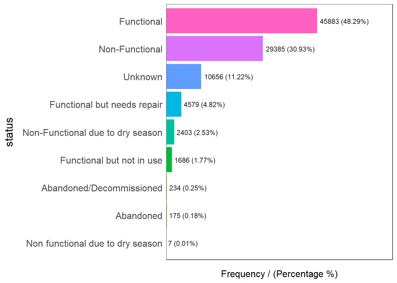
                            status frequency percentage cumulative_perc
1                       Functional     45883      48.29           48.29
2                   Non-Functional     29385      30.93           79.22
3                          Unknown     10656      11.22           90.44
4      Functional but needs repair      4579       4.82           95.26
5 Non-Functional due to dry season      2403       2.53           97.79
6        Functional but not in use      1686       1.77           99.56
7         Abandoned/Decommissioned       234       0.25           99.81
8                        Abandoned       175       0.18           99.99
9 Non functional due to dry season         7       0.01          100.00
Nigeria consists of almost 48% of functional, 30% of non-functional and 11% of unknown waterpoints.
freq(data=wp_sfT,
     input = 'water_tech')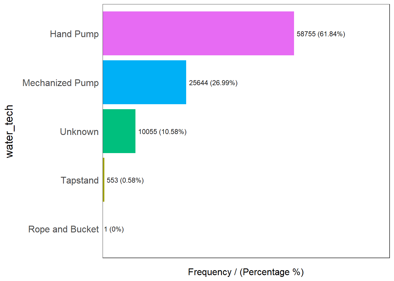
       water_tech frequency percentage cumulative_perc
1       Hand Pump     58755      61.84           61.84
2 Mechanized Pump     25644      26.99           88.83
3         Unknown     10055      10.58           99.41
4        Tapstand       553       0.58           99.99
5 Rope and Bucket         1       0.00          100.00
Nigeria consists of about majority of 61% of hand pump, 26% of mechanized pump and 10% of unknown water technology.
freq(data=wp_sfT,
     input = 'is_urban')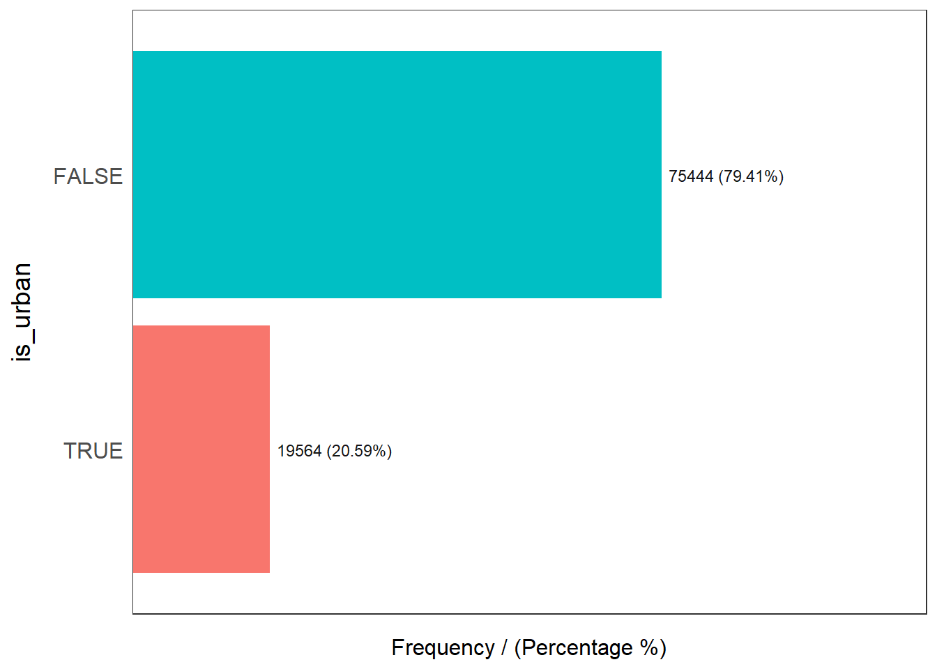
  is_urban frequency percentage cumulative_perc
1    FALSE     75444      79.41           79.41
2     TRUE     19564      20.59          100.00
Nigeria consists of about majority of 79% of rural regions, 20% of urban regions.
Histogram
Histogram is useful to identify the overall distribution of the data values (i.e. left skew, right skew or normal distribution)
The distribution of waterpoint proportion attributes
The code chunks below are used to create multiple histograms to reveal the overall distribution of the selected variables in nga_wp_clus.
pct_functional <- ggplot(data=nga_sf,
             aes(x= `pct_functional`)) +
  geom_histogram(bins=20,
                 color="black",
                 fill="light blue")

pct_nonfunctional <- ggplot(data=nga_sf,
             aes(x= `pct_nonfunctional`)) +
  geom_histogram(bins=20,
                 color="black",
                 fill="light blue")

pct_handpump <- ggplot(data=nga_sf,
             aes(x= `pct_handpump`)) +
  geom_histogram(bins=20,
                 color="black",
                 fill="light blue")

pct_usageCap1k <- ggplot(data=nga_sf,
             aes(x= `pct_usage1k`)) +
  geom_histogram(bins=20,
                 color="black",
                 fill="light blue")

pct_usageCapLess1k <- ggplot(data=nga_sf,
             aes(x= `pct_usageL1k`)) +
  geom_histogram(bins=20,
                 color="black",
                 fill="light blue")

pct_ruralWP <- ggplot(data=nga_sf,
             aes(x= `pct_ruralWP`)) +
  geom_histogram(bins=20,
                 color="black",
                 fill="light blue")

ggarrange(pct_functional, pct_nonfunctional, pct_handpump, pct_usageCap1k, pct_usageCapLess1k, pct_ruralWP,
          ncol = 3,
          nrow = 2)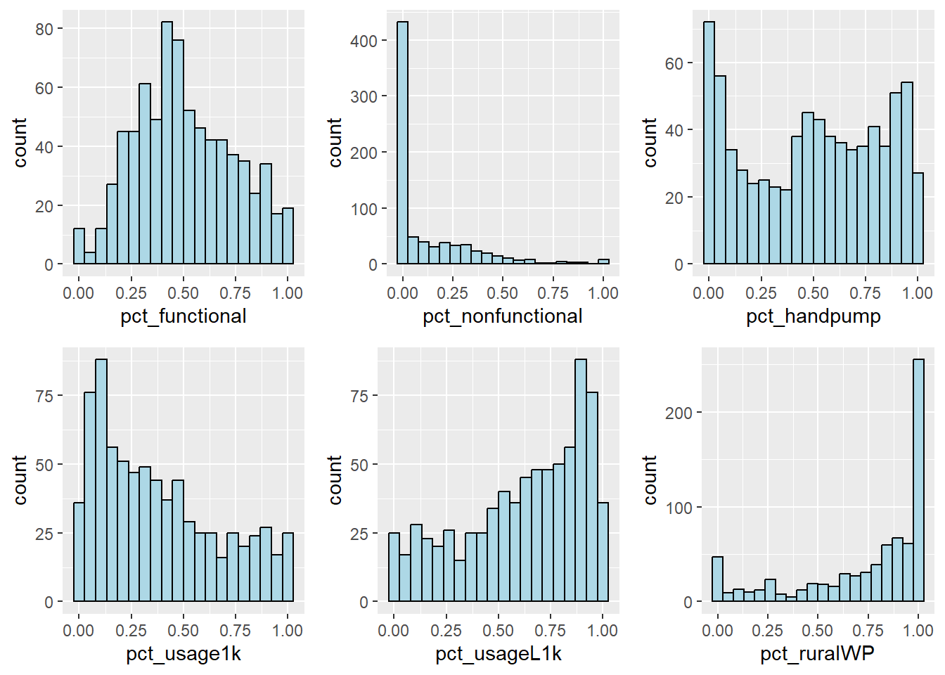
EDA using choropleth map
tm_shape(nga_sf) +
    tm_polygons(c("pct_functional", "pct_nonfunctional", "pct_handpump","pct_usage1k","pct_usageL1k", "pct_ruralWP"),
                style="jenks") +
    tm_facets(sync = TRUE, ncol = 2, nrow = 3) +
  tm_legend(legend.position = c("right", "bottom"), legend.title.size = 1.5,legend.text.size = 1)+
  tm_layout(outer.margins=0, asp=0)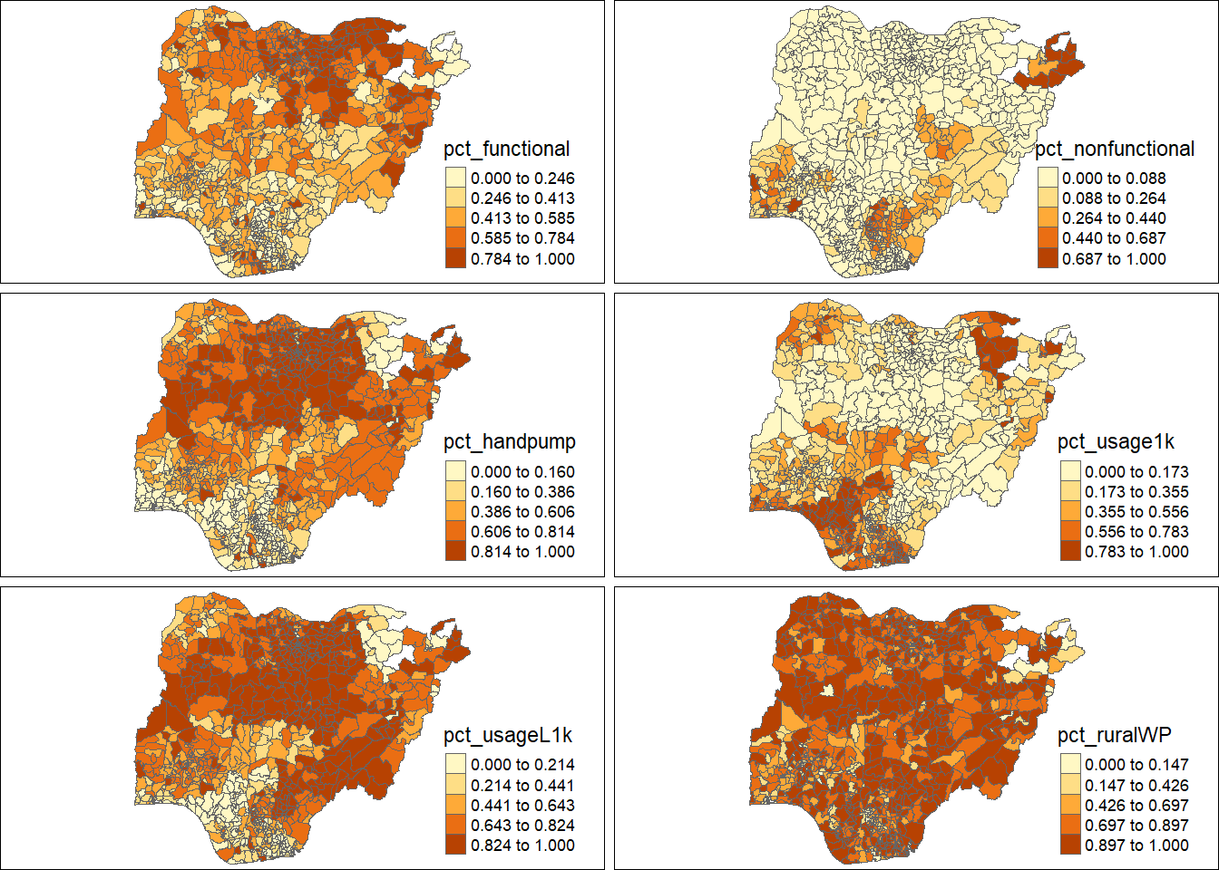
Correlation Analysis
Before we perform cluster analysis, it it important for us to ensure that the cluster variables are not highly correlated.
The code chunk below is used to visualise and analyse the correlation of the input variables.
str(nga_sf)Classes 'sf' and 'data.frame': 761 obs. of 16 variables:
$ shapeName : chr "aba north" "aba south" "abaji" "abak" ...
$ geometry :sfc_MULTIPOLYGON of length 761; first list element: List of 1
..$ :List of 1
.. ..$ : num [1:71, 1:2] 552560 552452 552269 552016 551706 ...
..- attr(*, "class")= chr [1:3] "XY" "MULTIPOLYGON" "sfg"
$ WPCount : int 17 71 57 48 233 34 119 152 66 39 ...
$ functional : int 7 29 23 23 82 16 72 79 18 25 ...
$ nonfunctional : int 1 7 0 0 109 3 14 11 22 1 ...
$ unknown_wp : int 9 35 34 25 42 15 33 62 26 13 ...
$ handpump : int 2 7 23 4 102 5 20 91 1 12 ...
$ usage1k : int 14 62 34 44 22 26 84 50 43 26 ...
$ usageL1k : int 3 9 23 4 211 8 35 102 23 13 ...
$ ruralWP : int 0 4 48 40 204 7 0 145 48 21 ...
$ pct_functional : num 0.412 0.408 0.404 0.479 0.352 ...
$ pct_nonfunctional: num 0.0588 0.0986 0 0 0.4678 ...
$ pct_handpump : num 0.1176 0.0986 0.4035 0.0833 0.4378 ...
$ pct_usage1k : num 0.8235 0.8732 0.5965 0.9167 0.0944 ...
$ pct_usageL1k : num 0.1765 0.1268 0.4035 0.0833 0.9056 ...
$ pct_ruralWP : num 0 0.0563 0.8421 0.8333 0.8755 ...
- attr(*, "sf_column")= chr "geometry"
- attr(*, "agr")= Factor w/ 3 levels "constant","aggregate",..: NA NA NA NA NA NA NA NA NA NA ...
..- attr(*, "names")= chr [1:15] "shapeName" "WPCount" "functional" "nonfunctional" ...nga_sf_var <- nga_sf %>%
st_drop_geometry() %>%
select("shapeName", "functional","nonfunctional", "pct_functional", "pct_nonfunctional", "pct_handpump","pct_usage1k","pct_usageL1k", "pct_ruralWP")
cluster_vars.cor = cor(nga_sf_var[,2:8])
corrplot.mixed(cluster_vars.cor,
lower = "ellipse",
upper = "number",
tl.pos = "lt",
diag = "l",
tl.col = "blue")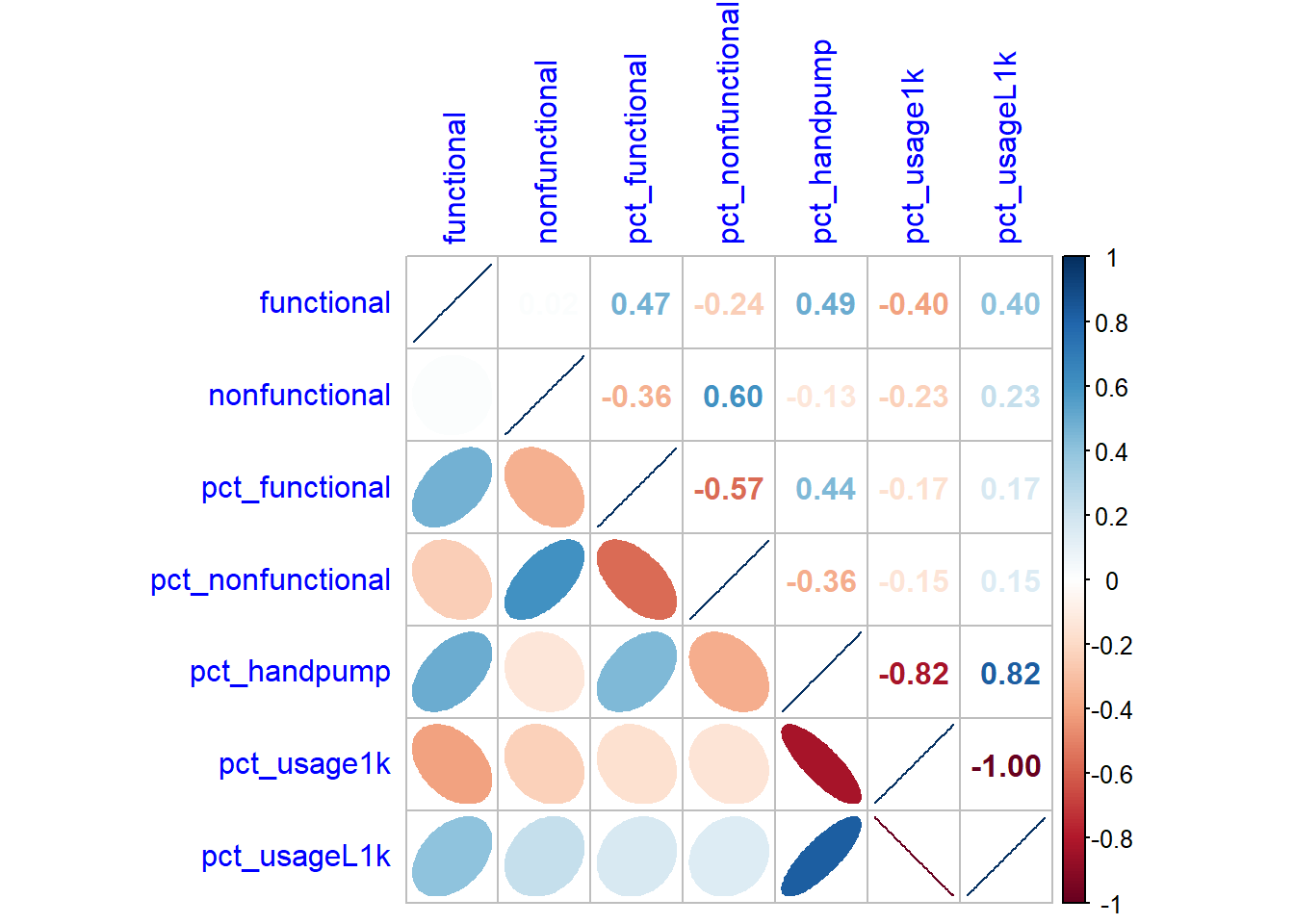
Hierarchy Cluster Analysis
The code chunk below will be used to extract the clustering variables from the nga_sf simple feature object into data.frame.
cluster_vars <- nga_sf_var %>%
  select("shapeName", "pct_functional", "pct_nonfunctional", "pct_handpump", "pct_usageL1k", "pct_ruralWP")
head(cluster_vars,10)
shapeName pct_functional pct_nonfunctional pct_handpump pct_usageL1k
1 aba north 0.4117647 0.05882353 0.11764706 0.17647059
2 aba south 0.4084507 0.09859155 0.09859155 0.12676056
4 abaji 0.4035088 0.00000000 0.40350877 0.40350877
5 abak 0.4791667 0.00000000 0.08333333 0.08333333
6 abakaliki 0.3519313 0.46781116 0.43776824 0.90557940
7 abeokuta north 0.4705882 0.08823529 0.14705882 0.23529412
8 abeokuta south 0.6050420 0.11764706 0.16806723 0.29411765
9 abi 0.5197368 0.07236842 0.59868421 0.67105263
10 aboh-mbaise 0.2727273 0.33333333 0.01515152 0.34848485
11 abua/odual 0.6410256 0.02564103 0.30769231 0.33333333
pct_ruralWP
1 0.00000000
2 0.05633803
4 0.84210526
5 0.83333333
6 0.87553648
7 0.20588235
8 0.00000000
9 0.95394737
10 0.72727273
11 0.53846154cluster_vars.cor = cor(cluster_vars[,2:6])
corrplot.mixed(cluster_vars.cor,
lower = "ellipse",
upper = "number",
tl.pos = "lt",
diag = "l",
tl.col = "blue")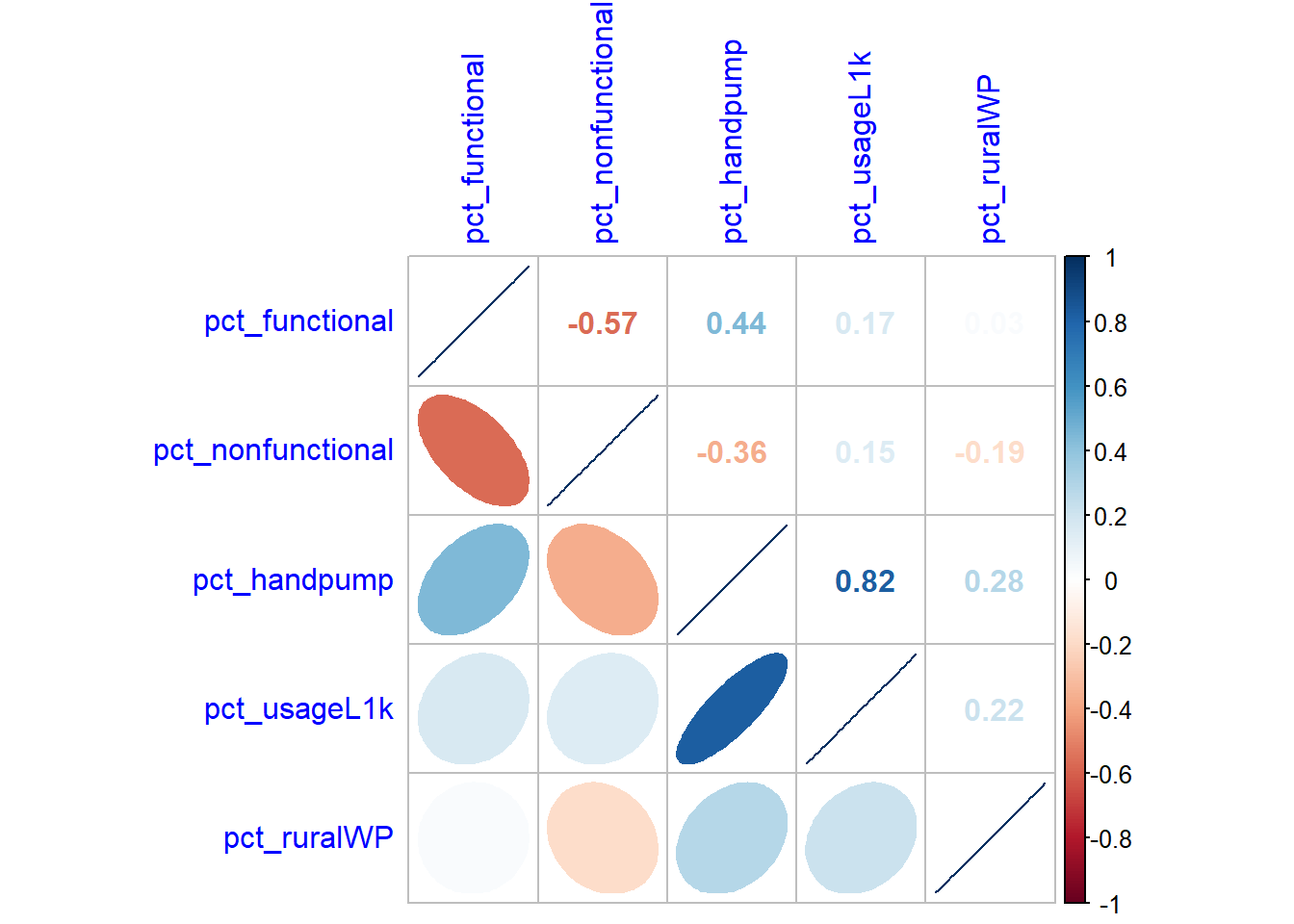
row.names(cluster_vars) <- cluster_vars$"shapeName"
head(cluster_vars,10)
shapeName pct_functional pct_nonfunctional pct_handpump
aba north aba north 0.4117647 0.05882353 0.11764706
aba south aba south 0.4084507 0.09859155 0.09859155
abaji abaji 0.4035088 0.00000000 0.40350877
abak abak 0.4791667 0.00000000 0.08333333
abakaliki abakaliki 0.3519313 0.46781116 0.43776824
abeokuta north abeokuta north 0.4705882 0.08823529 0.14705882
abeokuta south abeokuta south 0.6050420 0.11764706 0.16806723
abi abi 0.5197368 0.07236842 0.59868421
aboh-mbaise aboh-mbaise 0.2727273 0.33333333 0.01515152
abua/odual abua/odual 0.6410256 0.02564103 0.30769231
pct_usageL1k pct_ruralWP
aba north 0.17647059 0.00000000
aba south 0.12676056 0.05633803
abaji 0.40350877 0.84210526
abak 0.08333333 0.83333333
abakaliki 0.90557940 0.87553648
abeokuta north 0.23529412 0.20588235
abeokuta south 0.29411765 0.00000000
abi 0.67105263 0.95394737
aboh-mbaise 0.34848485 0.72727273
abua/odual 0.33333333 0.53846154nga_cluster_var <- select(cluster_vars, c(2:6))
head(nga_cluster_var, 10) pct_functional pct_nonfunctional pct_handpump pct_usageL1k
aba north 0.4117647 0.05882353 0.11764706 0.17647059
aba south 0.4084507 0.09859155 0.09859155 0.12676056
abaji 0.4035088 0.00000000 0.40350877 0.40350877
abak 0.4791667 0.00000000 0.08333333 0.08333333
abakaliki 0.3519313 0.46781116 0.43776824 0.90557940
abeokuta north 0.4705882 0.08823529 0.14705882 0.23529412
abeokuta south 0.6050420 0.11764706 0.16806723 0.29411765
abi 0.5197368 0.07236842 0.59868421 0.67105263
aboh-mbaise 0.2727273 0.33333333 0.01515152 0.34848485
abua/odual 0.6410256 0.02564103 0.30769231 0.33333333
pct_ruralWP
aba north 0.00000000
aba south 0.05633803
abaji 0.84210526
abak 0.83333333
abakaliki 0.87553648
abeokuta north 0.20588235
abeokuta south 0.00000000
abi 0.95394737
aboh-mbaise 0.72727273
abua/odual 0.53846154Data Standardization Standardization as it can handle outliers well and it is applicable to variables which are from normal distribution Z-score
nga_cluster_var.std <- normalize(nga_cluster_var)
summary(nga_cluster_var.std)
pct_functional pct_nonfunctional pct_handpump pct_usageL1k
Min. :0.0000 Min. :0.0000 Min. :0.0000 Min. :0.0000
1st Qu.:0.3333 1st Qu.:0.0000 1st Qu.:0.1860 1st Qu.:0.4157
Median :0.4792 Median :0.0000 Median :0.5255 Median :0.6807
Mean :0.5070 Mean :0.1277 Mean :0.4956 Mean :0.6182
3rd Qu.:0.6749 3rd Qu.:0.2105 3rd Qu.:0.7857 3rd Qu.:0.8750
Max. :1.0000 Max. :1.0000 Max. :1.0000 Max. :1.0000
pct_ruralWP
Min. :0.0000
1st Qu.:0.5922
Median :0.8717
Mean :0.7395
3rd Qu.:1.0000
Max. :1.0000 nga_cluster_var.z <- scale(nga_cluster_var)
describe(nga_cluster_var.z) vars n mean sd median trimmed mad min max range skew
pct_functional 1 761 0 1 -0.12 -0.03 1.04 -2.16 2.10 4.25 0.21
pct_nonfunctional 2 761 0 1 -0.62 -0.22 0.00 -0.62 4.27 4.89 1.98
pct_handpump 3 761 0 1 0.09 0.01 1.34 -1.53 1.56 3.09 -0.11
pct_usageL1k 4 761 0 1 0.22 0.09 1.07 -2.13 1.31 3.44 -0.60
pct_ruralWP 5 761 0 1 0.42 0.17 0.60 -2.35 0.83 3.18 -1.17
kurtosis se
pct_functional -0.67 0.04
pct_nonfunctional 4.04 0.04
pct_handpump -1.31 0.04
pct_usageL1k -0.80 0.04
pct_ruralWP 0.10 0.04Visualising the standardised clustering variables
Before performing clustering analysis, it is good to visualise the distribution of variables.
r <- ggplot(data=nga_sf,
             aes(x= `pct_functional`)) +
  geom_histogram(bins=20,
                 color="blue",
                 fill="#E69F00") +
  ggtitle("Raw values without standardisation")

nga_cluster_s_df <- as.data.frame(nga_cluster_var.std)
s <- ggplot(data=nga_cluster_s_df,
       aes(x=`pct_functional`)) +
  geom_histogram(bins=20,
                 color="blue",
                 fill="#E69F00") +
  ggtitle("Min-Max Standardisation")

nga_cluster_z_df <- as.data.frame(nga_cluster_var.z)
z <- ggplot(data=nga_cluster_z_df,
       aes(x=`pct_functional`)) +
  geom_histogram(bins=20,
                 color="blue",
                 fill="#E69F00") +
  ggtitle("Z-score Standardisation")

ggarrange(r, s, z,
          ncol = 3,
          nrow = 1)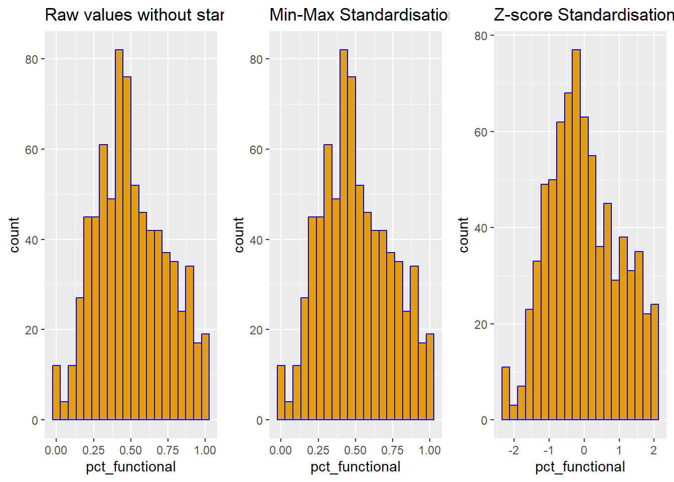
Computing Proximity Matrix
A proximity matrix is a square matrix (two-dimensional array) containing the distances, taken pairwise between the elements of a matrix. Broadly defined; a proximity matrix measures the similarity or dissimilarity between the pairs of matrix.
proxmat <- dist(nga_cluster_var, method = 'euclidean')Computing hierarchical clustering
hclust() can be used to perform hierarchical clustering. It supports eight clustering algorithms: ward.D, ward.D2, single, complete, average(UPGMA), mcquitty(WPGMA), median(WPGMC) and centroid(UPGMC).
The code chunk below is used to compute hierarchical clustering and adopt centroid method.
hclust_ward <- hclust(proxmat, method = 'ward.D')Selecting the optimal clustering algorithm by hierarchical clustering
agnes() function of cluster package cane calculate the agglomerative coefficient, which measures the amount of clustering structure.
m <- c( "average", "single", "complete", "ward")
names(m) <- c( "average", "single", "complete", "ward")

ac <- function(x) {
  agnes(nga_cluster_var, method = x)$ac
}

map_dbl(m, ac)
average single complete ward
0.9320242 0.8841971 0.9557188 0.9930958 Determining Optimal Clusters
There are three ways to determine the optimal clusters.
Elbow method
Average Silhouette Method
Gap Statistic Method
We are going to adopt Gap Statistic Method to determine the optimal clusters. The gap statistic compares the total within intra-cluster variation for different values of k with their expected values under null reference distribution of the data. The estimate of the optimal clusters will be value that maximize the gap statistic. This means that the clustering structure is far away from the random uniform distribution of points.
set.seed(1234)
gap_stat <- clusGap(nga_cluster_var,
                    FUN = hcut,
                    nstart = 25,
                    K.max = 10,
                    B = 50)
# Print the result
print(gap_stat, method = "firstmax")
Clustering Gap statistic ["clusGap"] from call:
clusGap(x = nga_cluster_var, FUNcluster = hcut, K.max = 10, B = 50, nstart = 25)
B=50 simulated reference sets, k = 1..10; spaceH0="scaledPCA"
--> Number of clusters (method 'firstmax'): 5
logW E.logW gap SE.sim
[1,] 5.026463 5.468043 0.4415796 0.008773640
[2,] 4.784723 5.341867 0.5571439 0.013342806
[3,] 4.670536 5.257902 0.5873658 0.009107344
[4,] 4.588263 5.189318 0.6010551 0.009205690
[5,] 4.464084 5.136493 0.6724086 0.009032431
[6,] 4.420326 5.091754 0.6714280 0.008259398
[7,] 4.366689 5.051587 0.6848981 0.008286133
[8,] 4.333252 5.019084 0.6858326 0.008194347
[9,] 4.291669 4.993013 0.7013443 0.007706852
[10,] 4.251836 4.970142 0.7183058 0.007584662Then, we can visualize the cluster plots.
fviz_gap_stat(gap_stat)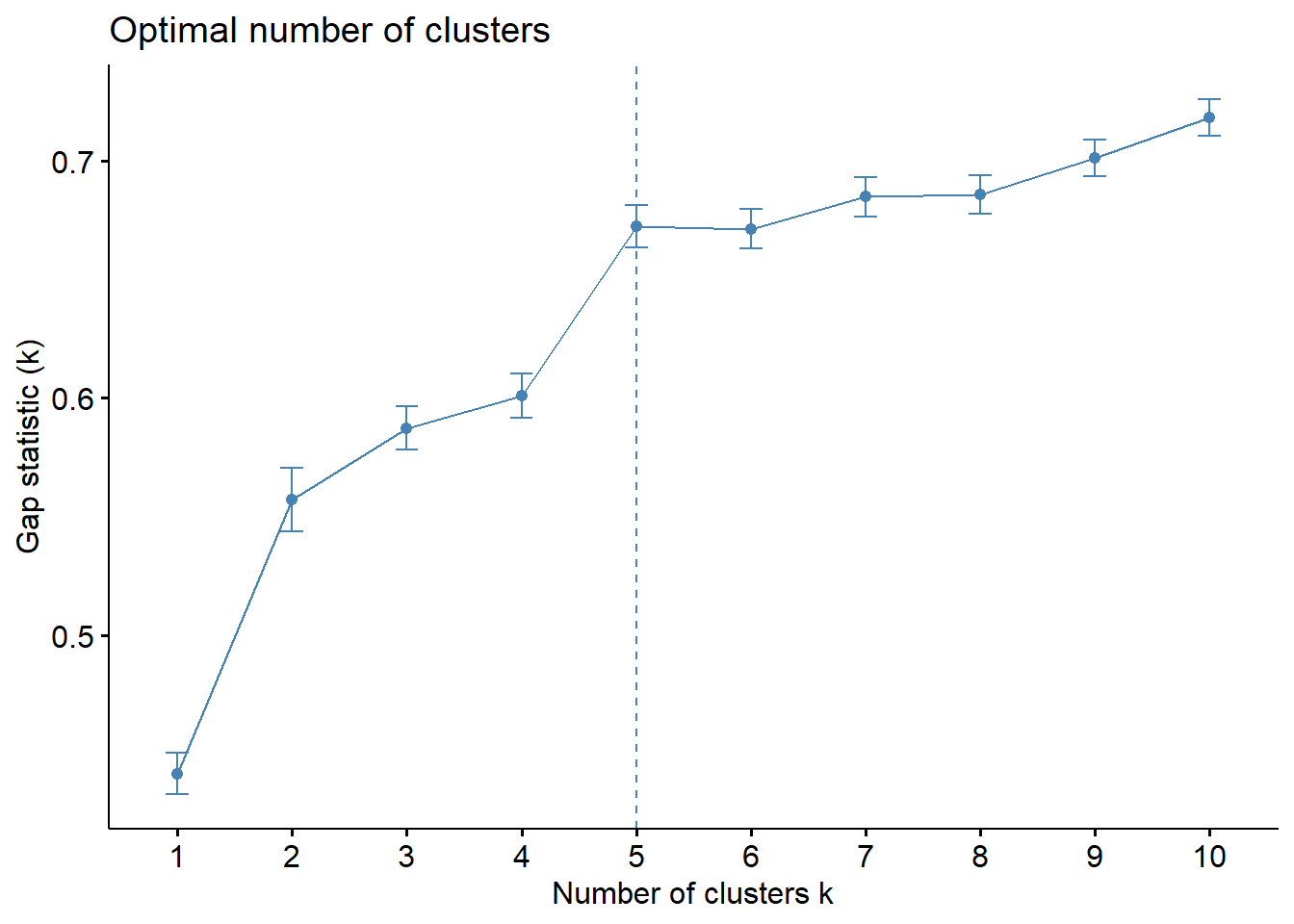
Interpreting the dendrogram
plot(hclust_ward,cex=0.6)
rect.hclust(hclust_ward,
            k = 4,
            border = 2:5)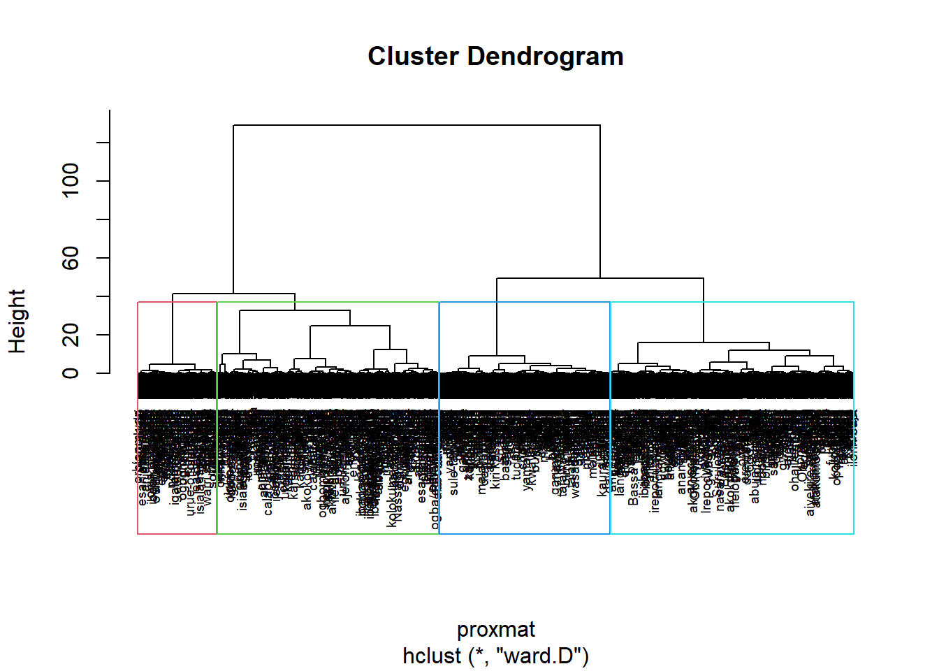
Visually-driven hierarchical clustering analysis
We are going to build both interactive and static cluster heatmaps with the help of heatmaply() package.
Transforming the data frame into a matrix
The code chunk below is used to transform lga_ict data frame into a data matrix.
nga_cluster_var_mat <- data.matrix(nga_cluster_var)Plotting Interactive Cluster Heatmap
heatmaply(normalize(nga_cluster_var_mat),
          Colv=NA,
          dist_method = "euclidean",
          hclust_method = "ward.D",
          seriate = "OLO",
          colors = Reds,
          k_row = 5,
          margins = c(NA,200,60,NA),
          fontsize_row = 4,
          fontsize_col = 5,
          main="Geographic Segmentation of Nigeria WP indicators",
          xlab = "ICT Indicators",
          ylab = "ShapeName"
          )
Mapping the clusters formed
The code chunk below is used to derive a 5-cluster model based on hierarchical clustering.
groups <- as.factor(cutree(hclust_ward, k=5))
nga_sf_cluster <- cbind(nga_sf, as.matrix(groups)) %>%
  rename(`CLUSTER`=`as.matrix.groups.`)
qtm(nga_sf_cluster, "CLUSTER")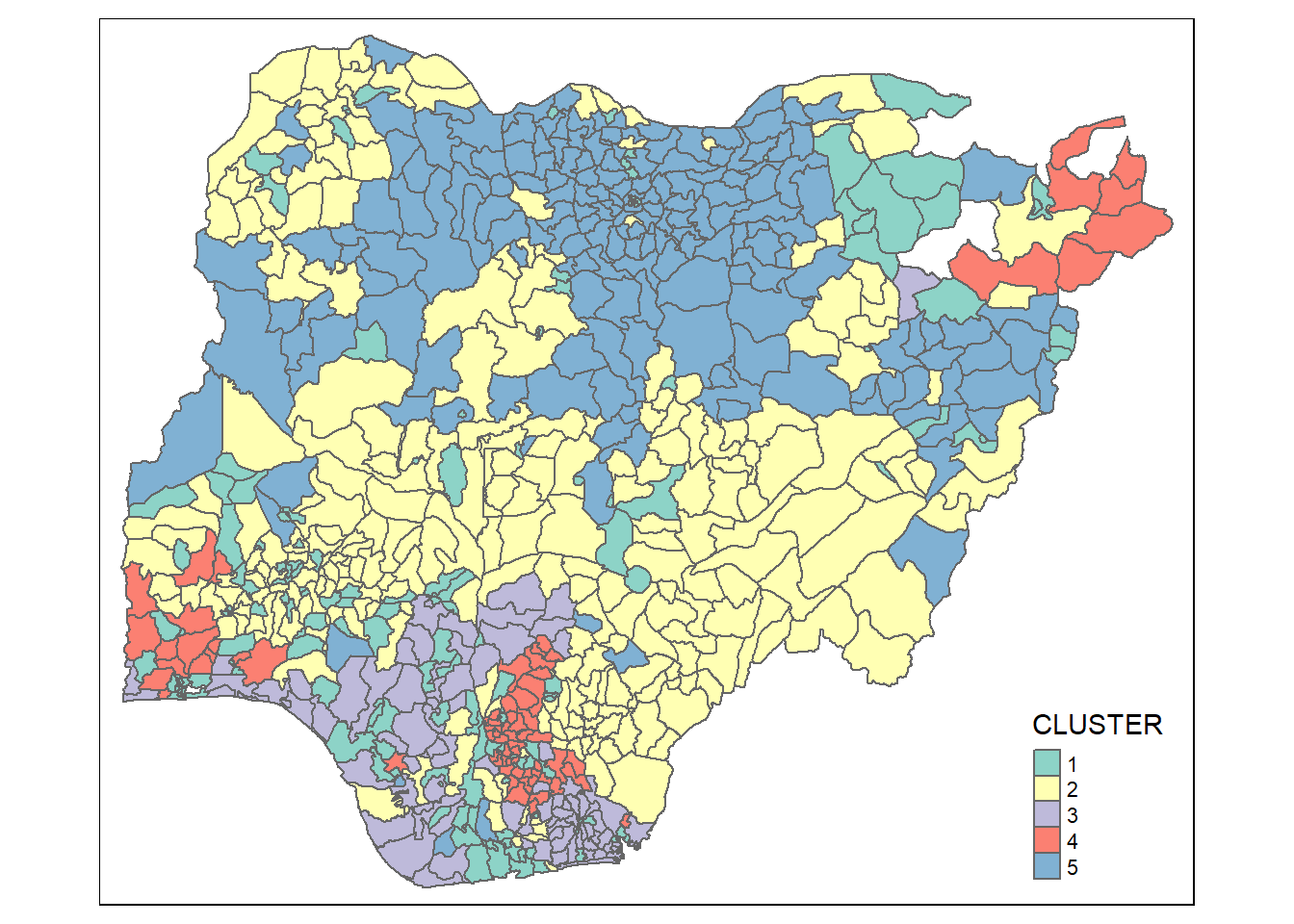
Elbow Method
The Elbow Method looks at the total WSS(within-cluster sum of Square) as a function of the number clusters.
set.seed(1234)
# function to compute total within-cluster sum of squares
fviz_nbclust(nga_cluster_var, hcut, method = "wss", k.max = 10) + theme_minimal() + ggtitle("the Elbow Method")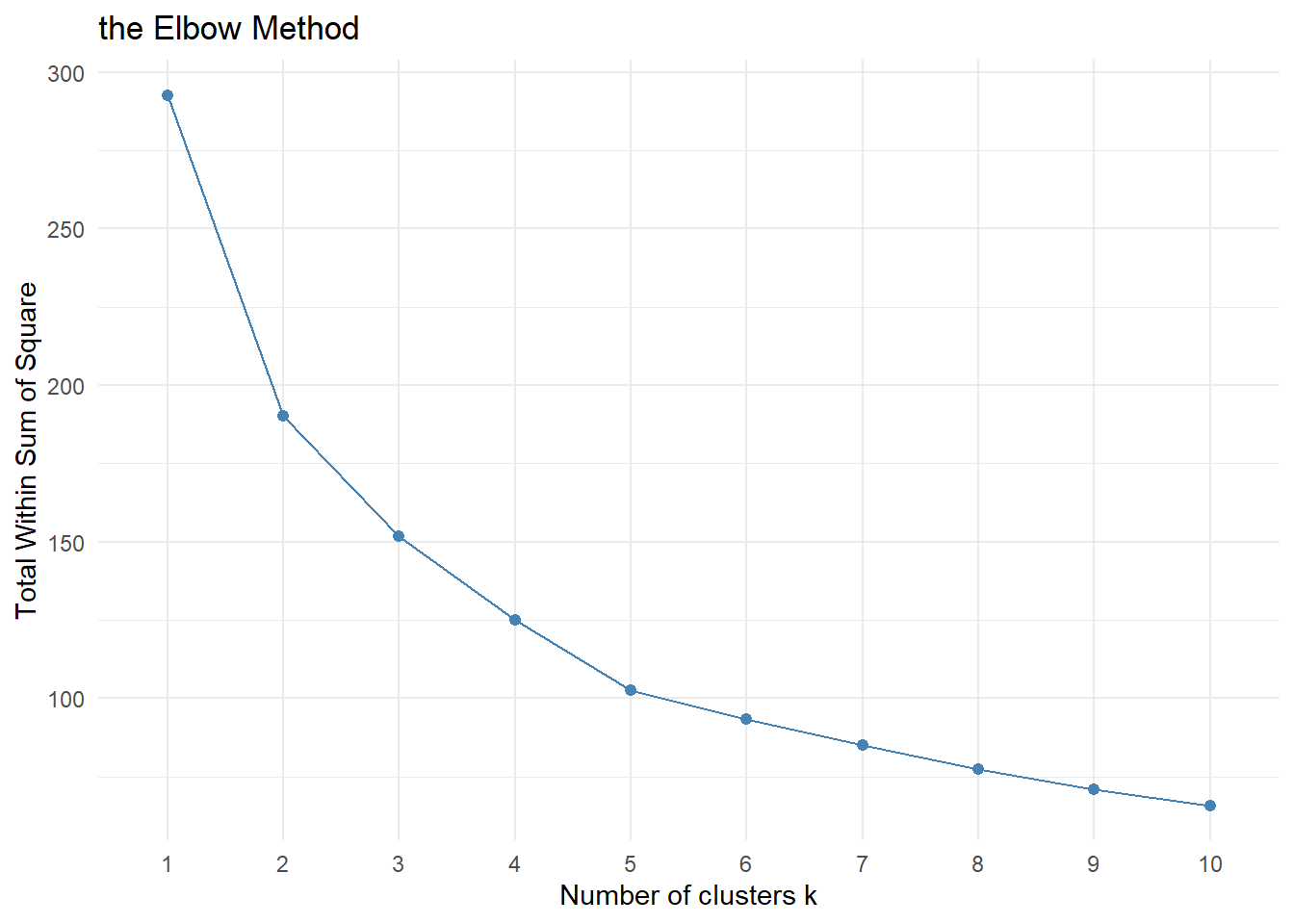
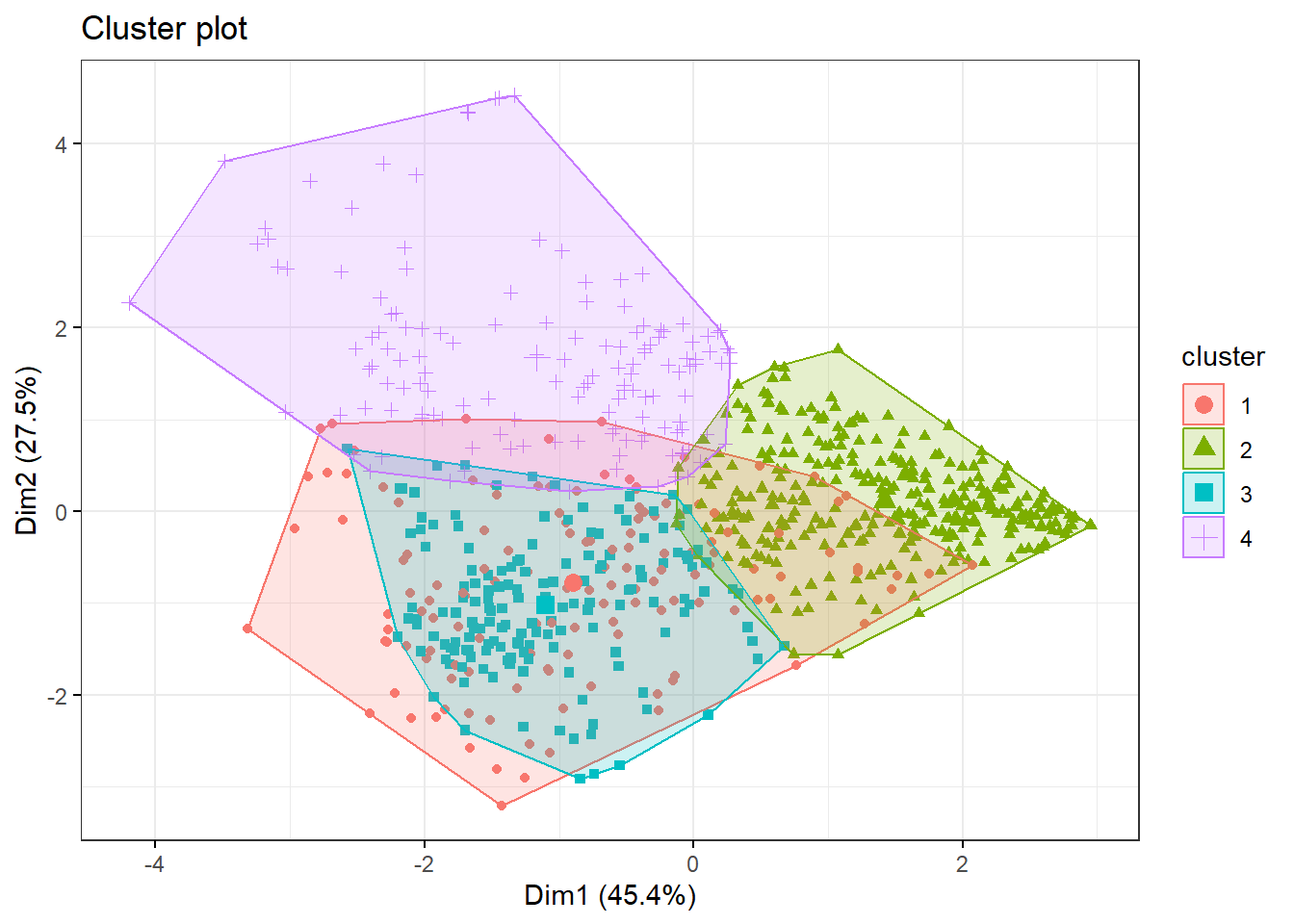
Plot K-means
kmm <- kmeans(nga_cluster_var,4,nstart = 25)
fviz_cluster(kmm, data = nga_cluster_var,
             geom = "point",
             ellipse.type = "convex",
             ggtheme = theme_bw()
             )
Multivariate Visualisation
Past studies shown that parallel coordinate plot can be used to reveal clustering variables by cluster very effectively. In the code chunk below, ggparcoord() of GGally package
ggparcoord(data = nga_sf_cluster,
           columns = c(10:15),
           groupColumn = "CLUSTER",
           scale = "std",
           alphaLines = 0.2,
           boxplot = TRUE,
           title = "Multiple Parallel Coordinates Plots of Nigeria Variables by Cluster") +
  facet_grid(~ CLUSTER) +
  theme(axis.text.x = element_text(angle = 30, size = 15)) +
  scale_color_viridis(option = "C", discrete=TRUE)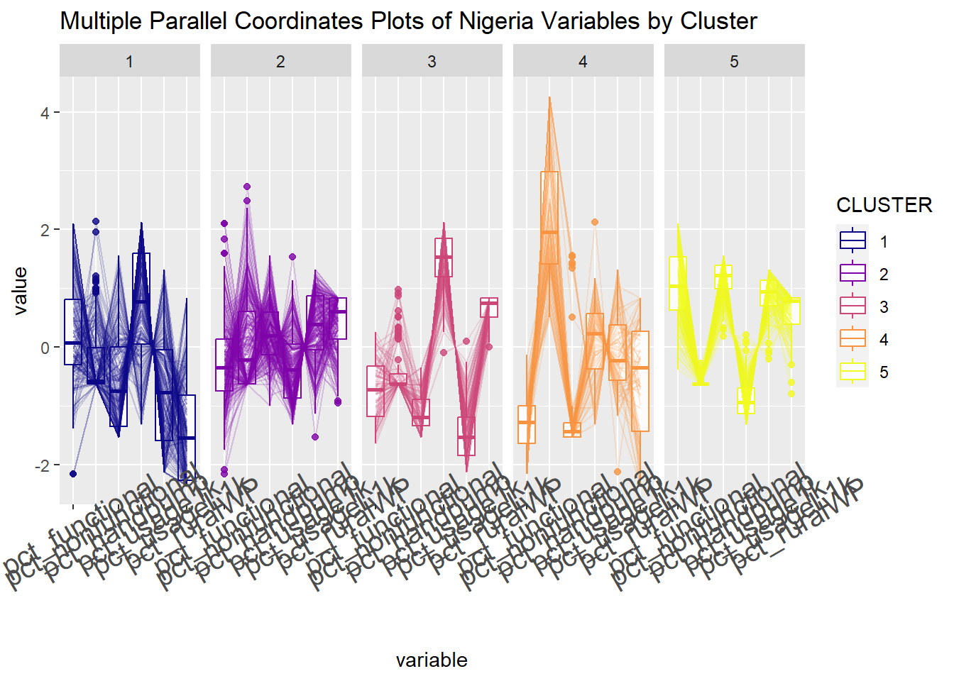
In the code chunk below, group_by() and summarise() of dplyr are used to derive mean values of the clustering variables.
nga_sf_cluster %>%
  st_set_geometry(NULL) %>%
  group_by(CLUSTER) %>%
  summarise(mean_pct_functional = mean(pct_functional),
            mean_pct_nonfunctional = mean(pct_nonfunctional),
            mean_pct_handpump = mean(pct_handpump),
            mean_pct_usage1k = mean(pct_usage1k),
            mean_pct_usageL1k = mean(pct_usageL1k),
            mean_pct_ruralWP = mean(pct_ruralWP))
# A tibble: 5 × 7
CLUSTER mean_pct_functional mean_pct_nonfunc…¹ mean_…² mean_…³ mean_…⁴ mean_…⁵
<chr> <dbl> <dbl> <dbl> <dbl> <dbl> <dbl>
1 1 0.571 0.0847 0.311 0.600 0.400 0.299
2 2 0.440 0.144 0.574 0.281 0.719 0.871
3 3 0.334 0.0426 0.134 0.809 0.191 0.943
4 4 0.195 0.575 0.113 0.407 0.593 0.567
5 5 0.750 0.00218 0.871 0.123 0.877 0.922
# … with abbreviated variable names ¹mean_pct_nonfunctional,
# ²mean_pct_handpump, ³mean_pct_usage1k, ⁴mean_pct_usageL1k,
# ⁵mean_pct_ruralWPComputing spatially constrained clusters using SKATER method
The code chunk below is used to compute the spatially constrained clusters using as_Spatial() of poly2nd( ) packages.
nga_sp <- as_Spatial(nga_sf)nga.nb <- poly2nb(nga_sp, queen=TRUE)
summary(nga.nb)Neighbour list object:
Number of regions: 761
Number of nonzero links: 4348
Percentage nonzero weights: 0.750793
Average number of links: 5.713535
Link number distribution:
1 2 3 4 5 6 7 8 9 10 11 12 14
4 16 57 122 177 137 121 71 39 11 4 1 1
4 least connected regions:
138 509 525 560 with 1 link
1 most connected region:
508 with 14 linksnga.nb <- poly2nb(nga_sp, queen=TRUE)
summary(nga.nb)Neighbour list object:
Number of regions: 761
Number of nonzero links: 4348
Percentage nonzero weights: 0.750793
Average number of links: 5.713535
Link number distribution:
1 2 3 4 5 6 7 8 9 10 11 12 14
4 16 57 122 177 137 121 71 39 11 4 1 1
4 least connected regions:
138 509 525 560 with 1 link
1 most connected region:
508 with 14 linksComputing minimum spanning tree
The code chunk below is used to compute the cost of each edge.
lcosts <- nbcosts(nga.nb, nga_cluster_var)nga.w <- nb2listw(nga.nb,
lcosts,
style="B")
summary(nga.w)Characteristics of weights list object:
Neighbour list object:
Number of regions: 761
Number of nonzero links: 4348
Percentage nonzero weights: 0.750793
Average number of links: 5.713535
Link number distribution:

  1   2   3   4   5   6   7   8   9  10  11  12  14
  4  16  57 122 177 137 121  71  39  11   4   1   1
4 least connected regions:
138 509 525 560 with 1 link
1 most connected region:
508 with 14 links
Weights style: B
Weights constants summary:
n nn S0 S1 S2
B 761 579121 1989.853 2574.866 26667.43mstree() function of spdep packages can be used to compute minimum spanning tree.
nga.mst <- mstree(nga.w)We can have a look at the dimension of the MST.
dim(nga.mst)[1] 760 3We can plot the MST to show the observation numbers of the nodes along with the LGA boundaries.
plot(nga_sp, border=gray(.5))
plot.mst(nga.mst,
         coordinates(nga_sp),
         col="blue",
         cex.lab=0.7,
         cex.circles=0.005,
         add=TRUE)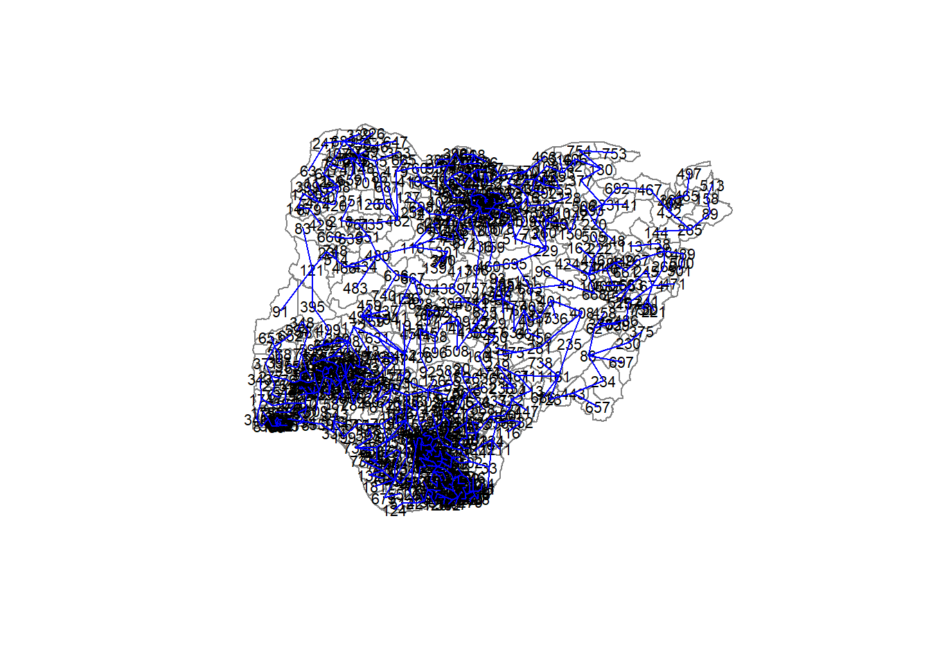
Computing spatially constrained clusters using SKATER method
The code chunk below is used to compute the spatially constrained clusters using skater() of spdep packages.
clust4 <- spdep::skater(edges = nga.mst[,1:2],
                 data = nga_cluster_var,
                 method = "euclidean",
ncuts = 4)str(clust4)List of 8
$ groups : num [1:761] 2 2 5 2 4 3 3 4 2 3 ...
$ edges.groups:List of 5
..$ :List of 3
.. ..$ node: num [1:208] 479 760 442 166 95 94 137 404 699 103 ...
.. ..$ edge: num [1:207, 1:3] 406 253 130 377 108 467 414 432 692 223 ...
.. ..$ ssw : num 87.1
..$ :List of 3
.. ..$ node: num [1:124] 33 102 65 101 332 717 539 214 9 359 ...
.. ..$ edge: num [1:123, 1:3] 9 359 538 214 539 717 332 101 65 102 ...
.. ..$ ssw : num 62.8
..$ :List of 3
.. ..$ node: num [1:161] 363 27 585 310 311 545 194 559 334 573 ...
.. ..$ edge: num [1:160, 1:3] 311 310 545 194 559 334 573 199 14 567 ...
.. ..$ ssw : num 85.1
..$ :List of 3
.. ..$ node: num [1:75] 234 723 443 161 711 461 413 722 408 727 ...
.. ..$ edge: num [1:74, 1:3] 13 564 533 408 455 215 491 401 281 408 ...
.. ..$ ssw : num 19.6
..$ :List of 3
.. ..$ node: num [1:193] 66 499 395 121 23 514 651 761 466 480 ...
.. ..$ edge: num [1:192, 1:3] 66 499 395 121 537 23 627 118 298 544 ...
.. ..$ ssw : num 81.4
$ not.prune : NULL
$ candidates : int [1:5] 1 2 3 4 5
$ ssto : num 441
$ ssw : num [1:5] 441 409 364 350 336
$ crit : num [1:2] 1 Inf
$ vec.crit : num [1:761] 1 1 1 1 1 1 1 1 1 1 ...
- attr(*, "class")= chr "skater"ccs4 <- clust4$groups
ccs4 [1] 2 2 5 2 4 3 3 4 2 3 5 5 4 3 5 3 4 2 5 4 3 2 5 2 3 3 3 3 5 3 3 1 2 3 1 3 5
[38] 5 3 5 2 3 5 5 5 1 5 3 1 3 3 3 2 2 2 3 3 5 3 4 3 1 5 5 2 5 3 1 5 5 3 3 5 1
[75] 4 2 2 2 3 1 3 1 5 1 1 5 1 1 1 4 5 5 4 1 1 1 1 1 1 4 2 2 1 5 1 1 5 1 1 5 5
[112] 1 1 5 1 4 4 5 3 3 5 5 5 3 1 5 1 1 5 1 4 3 5 2 2 5 1 1 5 1 1 1 1 1 1 5 5 5
[149] 1 1 1 1 1 1 3 3 1 1 1 5 4 1 2 1 1 1 2 4 5 5 5 5 5 3 3 3 5 3 2 5 3 2 5 5 5
[186] 5 2 3 2 5 2 2 2 3 3 3 3 3 3 2 2 2 3 3 3 2 2 3 3 3 4 3 2 2 4 4 1 5 1 1 1 1
[223] 1 5 1 5 1 1 1 1 1 1 1 4 4 1 5 4 1 1 1 5 2 1 1 5 5 1 4 1 5 5 1 1 1 5 5 1 5
[260] 1 1 4 4 1 1 1 1 1 3 3 3 3 3 3 3 3 3 3 2 2 4 2 3 5 2 2 2 2 3 5 3 5 5 5 5 5
[297] 5 5 5 3 5 3 2 2 2 3 2 2 3 3 3 3 5 5 2 3 3 1 2 3 3 5 5 4 2 3 2 2 3 3 4 2 5
[334] 3 5 5 5 5 5 5 5 5 3 1 2 3 3 3 5 5 5 3 5 5 3 4 4 2 2 2 5 2 3 3 3 2 1 3 2 2
[371] 3 3 4 5 1 1 1 1 1 5 5 1 1 4 4 4 5 1 5 5 5 1 1 5 5 1 3 1 5 1 4 1 4 1 1 1 1
[408] 4 5 1 5 1 4 1 5 1 5 1 4 5 5 2 1 1 1 1 1 5 5 5 3 1 4 5 3 1 1 5 1 1 1 1 4 1
[445] 5 1 4 5 1 5 3 3 3 1 4 4 5 1 5 1 4 5 1 1 1 5 1 1 1 1 1 5 1 5 1 1 4 1 1 5 1
[482] 5 5 1 1 1 2 2 1 1 4 1 1 2 5 5 1 5 5 1 1 1 3 5 1 1 1 5 5 3 3 3 1 5 2 1 1 2
[519] 2 4 2 2 2 2 2 2 2 2 1 2 3 4 4 4 2 3 5 2 2 4 4 3 3 5 3 2 5 3 3 2 3 3 5 5 5
[556] 4 3 2 3 2 2 2 4 4 4 2 3 4 5 5 5 2 3 2 3 4 3 3 3 5 3 3 3 2 3 5 5 4 2 3 2 2
[593] 3 3 3 5 5 2 5 2 2 2 2 2 2 2 3 3 3 3 2 5 4 3 3 3 3 2 2 2 5 5 2 3 3 3 5 5 4
[630] 3 5 3 1 4 5 5 1 3 5 1 1 1 4 1 1 5 5 5 1 3 5 3 3 1 5 3 4 3 5 5 1 1 1 4 1 1
[667] 5 1 3 5 1 5 5 1 3 1 5 1 5 3 5 5 1 2 1 4 5 5 5 1 4 1 1 1 1 5 1 1 1 1 5 2 2
[704] 3 2 3 3 2 3 2 4 2 2 3 2 2 2 1 2 2 2 4 4 3 2 2 4 5 5 1 1 3 3 3 5 4 1 4 5 5
[741] 5 5 5 4 4 1 1 5 3 1 1 1 1 1 1 1 1 5 1 1 5we can also plot the pruned tree that shows the five clusters on top of the admin 2 area.
plot(nga_sp, border=gray(.5))
plot(clust4,
     coordinates(nga_sp),
     cex.lab=.7,
     groups.colors=c("blue","red","brown", "green", "pink"),
     cex.circles=0.005,
     add=TRUE)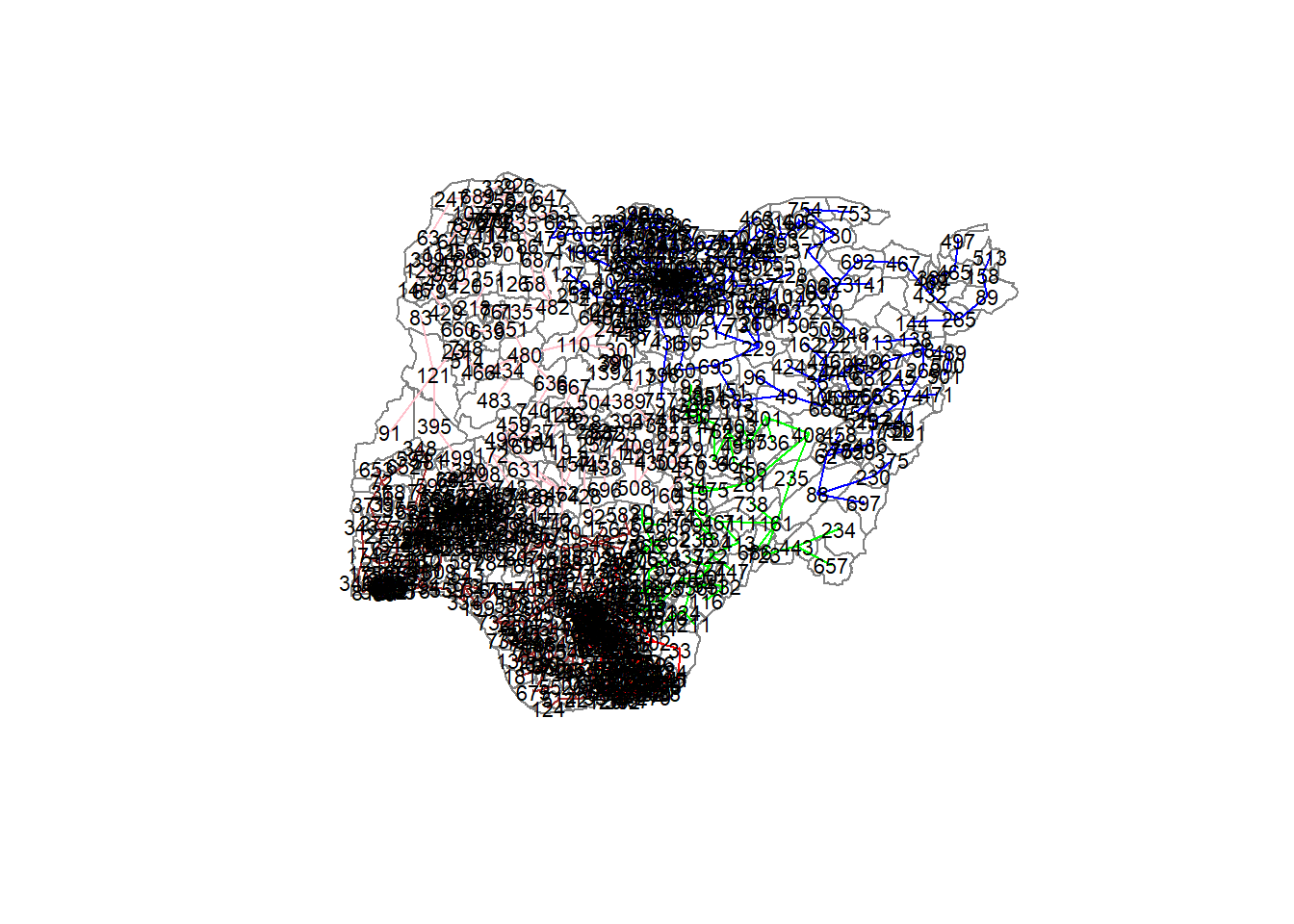
Visualising the clusters in choropleth map
The code chunk below is used to plot the clusters derived by SKATER method.
groups_mat <- as.matrix(clust4$groups)
nga_sf_spatialcluster <- cbind(nga_sf_cluster, as.factor(groups_mat)) %>%
  rename(`SP_CLUSTER`=`as.factor.groups_mat.`)
qtm(nga_sf_spatialcluster, "SP_CLUSTER")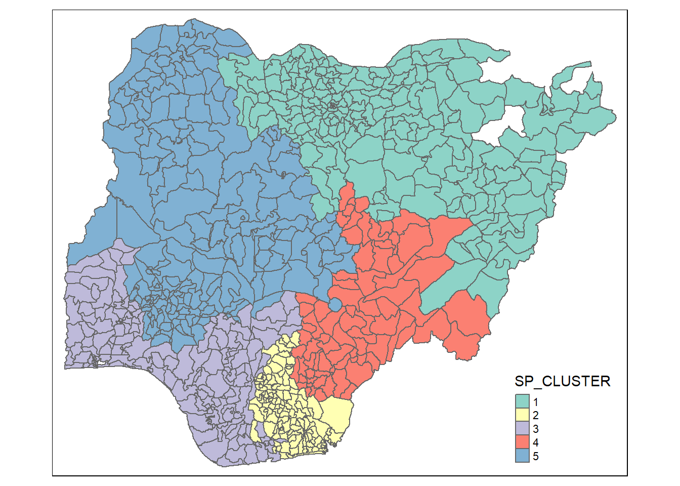
In the code chunk below, group_by() and summarise() of dplyr are used to derive mean values of the clustering variables.
nga_sf_spatialcluster %>%
  st_set_geometry(NULL) %>%
  group_by(SP_CLUSTER) %>%
  summarise(mean_pct_functional = mean(pct_functional),
            mean_pct_nonfunctional = mean(pct_nonfunctional),
            mean_pct_handpump = mean(pct_handpump),
            mean_pct_usage1k = mean(pct_usage1k),
            mean_pct_usageL1k = mean(pct_usageL1k),
            mean_pct_ruralWP = mean(pct_ruralWP))
# A tibble: 5 × 7
SP_CLUSTER mean_pct_functional mean_pct_nonf…¹ mean_…² mean_…³ mean_…⁴ mean_…⁵
<fct> <dbl> <dbl> <dbl> <dbl> <dbl> <dbl>
1 1 0.715 0.0427 0.778 0.215 0.785 0.806
2 2 0.307 0.282 0.145 0.572 0.428 0.698
3 3 0.449 0.150 0.218 0.615 0.385 0.619
4 4 0.361 0.266 0.590 0.146 0.854 0.921
5 5 0.516 0.0474 0.612 0.337 0.663 0.725
# … with abbreviated variable names ¹mean_pct_nonfunctional,
# ²mean_pct_handpump, ³mean_pct_usage1k, ⁴mean_pct_usageL1k,
# ⁵mean_pct_ruralWPPlace both the hierarchical clustering and spatially constrained hierarchical clustering maps next to each other.
hclust.map <- qtm(nga_sf_cluster,
                  "CLUSTER", title = "Hierarchical clustering") +
  tm_borders(alpha = 0.5)

shclust.map <- qtm(nga_sf_spatialcluster,
                   "SP_CLUSTER", title = "spatially constrained clusters using SKATER method") +
  tm_borders(alpha = 0.5)

tmap_arrange(hclust.map, shclust.map,
             asp=NA, ncol=2)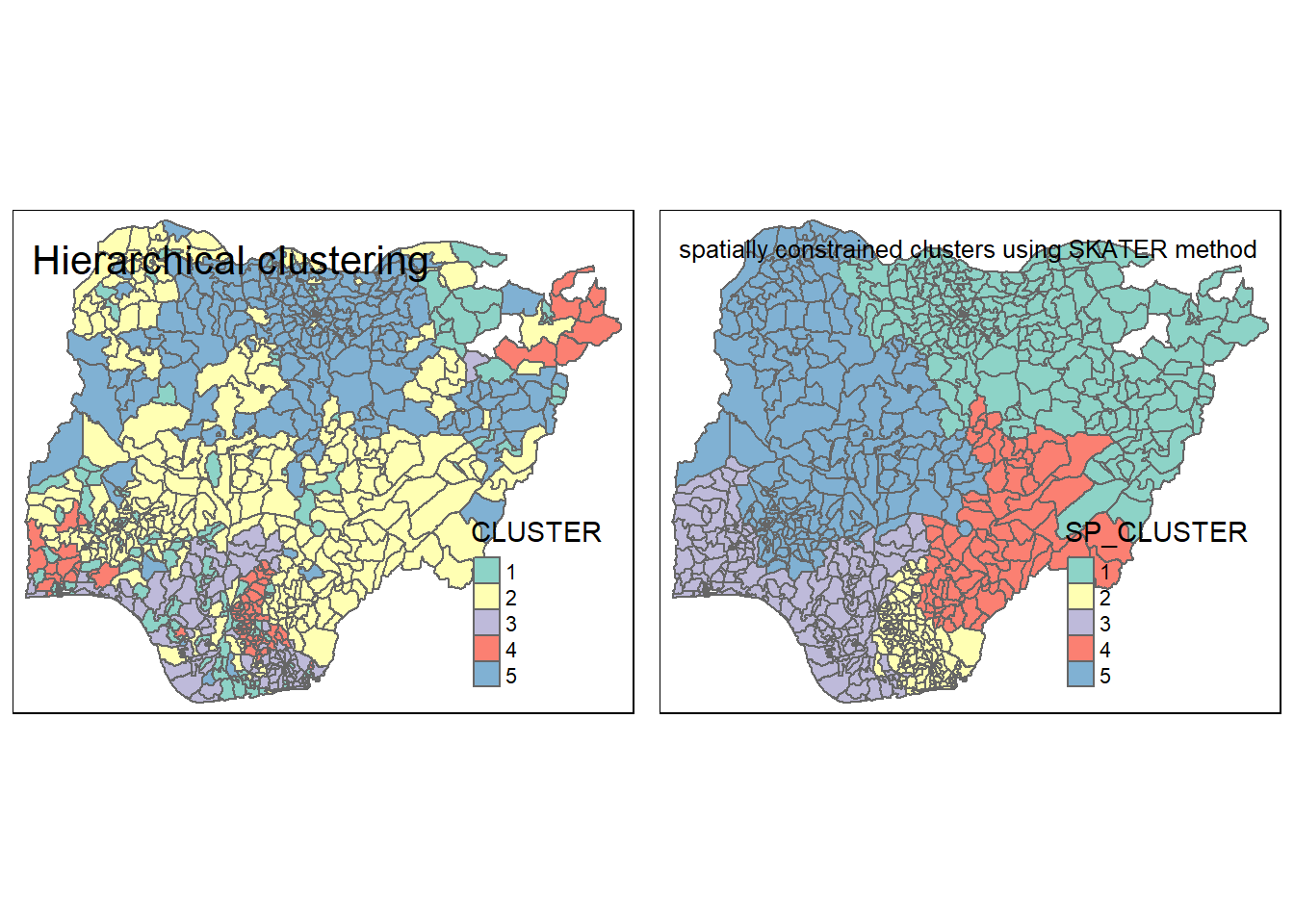
Spatially Constrained Clustering: ClustGeo Method
In this section, we are going to use ClustGeo package to perform non-spatially constrained hierarchical cluster analysis and spatially constrained cluster analysis.
Ward-like hierarchical clustering: ClustGeo
To perform non-spatially constrained hierarchical cluster, we only need to provide the function a dissimilarity matrix as shown in the code chunk below.
nongeo_cluster <- hclustgeo(proxmat)
plot(nongeo_cluster, cex = 0.5)
rect.hclust(nongeo_cluster,
            k = 5,
            border = 2:5)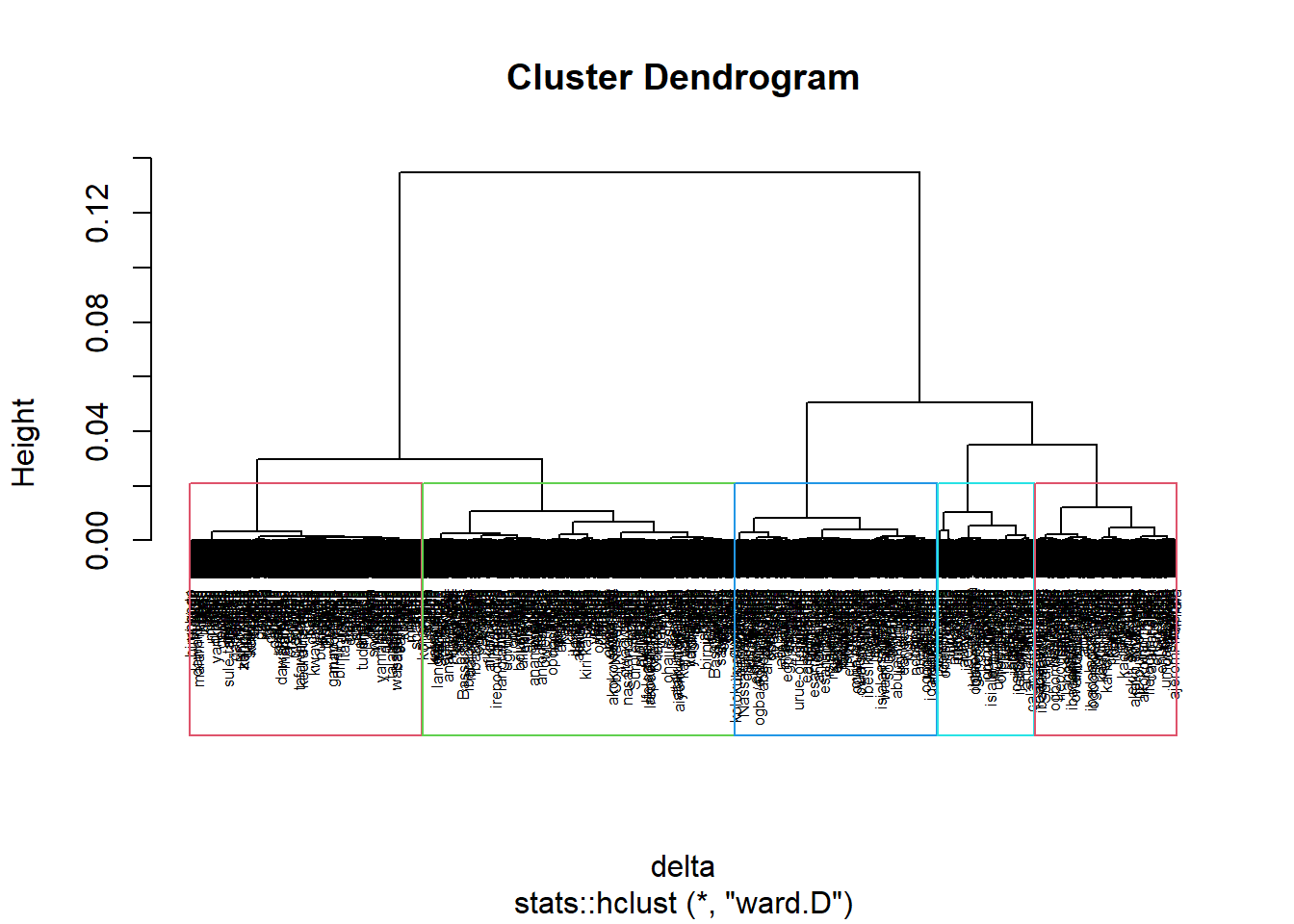
Mapping the clusters formed
groups <- as.factor(cutree(nongeo_cluster, k=5))
nga_sf_ngeo_cluster <- cbind(nga_sf, as.matrix(groups)) %>%
  rename(`CLUSTER` = `as.matrix.groups.`)
qtm(nga_sf_ngeo_cluster, "CLUSTER")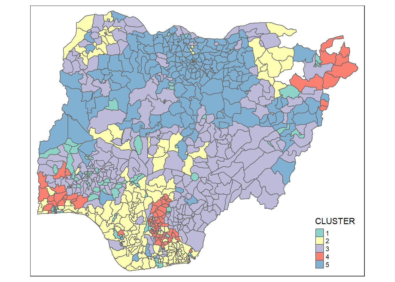
Spatially Constrained Clustering
A spatial distance matrix will be derived by using st_distance() of sf package before we perform spatially constrained hierarchical clustering.
dist <- st_distance(nga_sf, nga_sf)
distmat <- as.dist(dist)
cr <- choicealpha(proxmat, distmat, range.alpha = seq(0, 1, 0.1), K=5, graph = TRUE)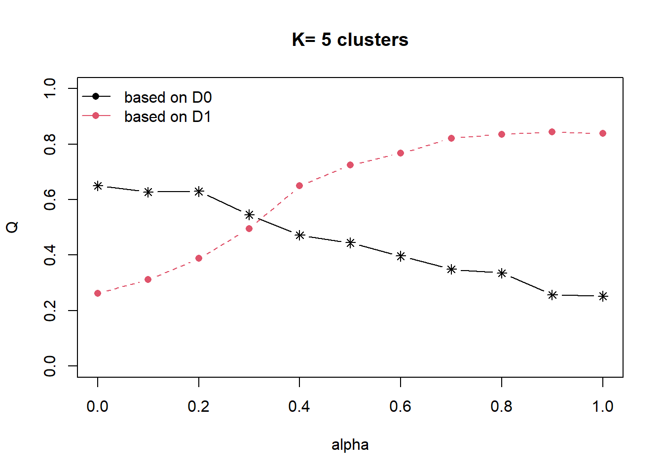
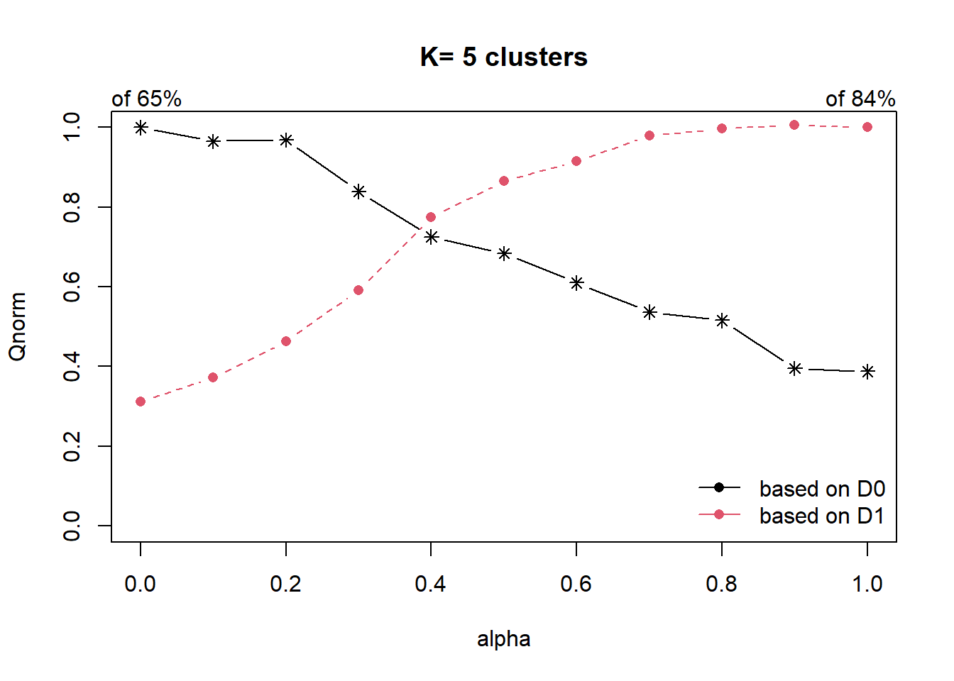
clustG <- hclustgeo(proxmat, distmat, alpha = 0.4)
groups <- as.factor(cutree(clustG, k=5))
nga_sf_Gcluster <- cbind(nga_sf, as.matrix(groups)) %>%
rename(`CLUSTER` = `as.matrix.groups.`)qtm(nga_sf_Gcluster, "CLUSTER")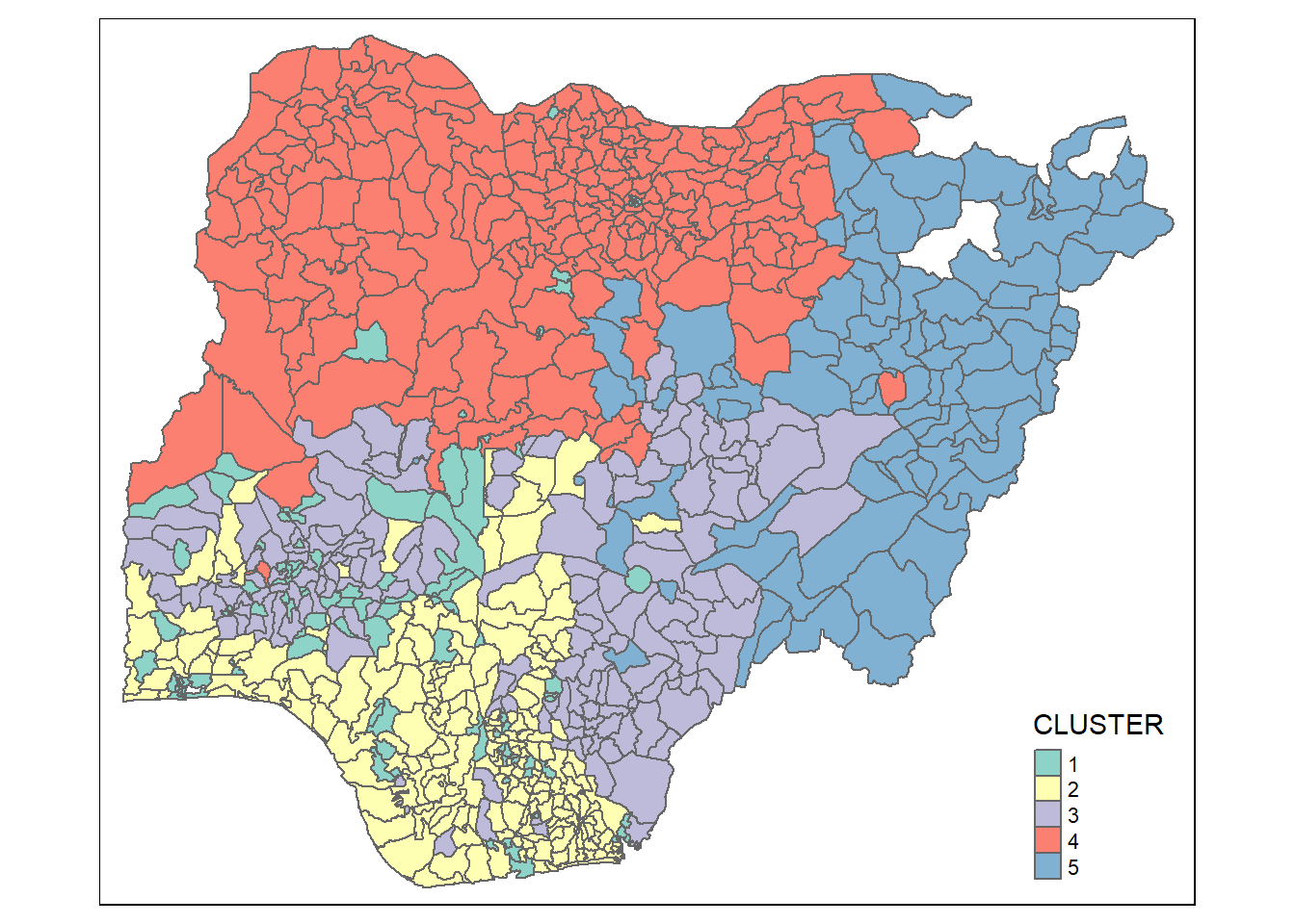
In the code chunk below, group_by() and summarise() of dplyr are used to derive mean values of the clustering variables.
nga_sf_Gcluster %>%
  st_set_geometry(NULL) %>%
  group_by(CLUSTER) %>%
  summarise(mean_pct_functional = mean(pct_functional),
            mean_pct_nonfunctional = mean(pct_nonfunctional),
            mean_pct_handpump = mean(pct_handpump),
            mean_pct_usage1k = mean(pct_usage1k),
            mean_pct_usageL1k = mean(pct_usageL1k),
            mean_pct_ruralWP = mean(pct_ruralWP))
# A tibble: 5 × 7
CLUSTER mean_pct_functional mean_pct_nonfunc…¹ mean_…² mean_…³ mean_…⁴ mean_…⁵
<chr> <dbl> <dbl> <dbl> <dbl> <dbl> <dbl>
1 1 0.540 0.117 0.363 0.509 0.491 0.191
2 2 0.344 0.200 0.147 0.643 0.357 0.803
3 3 0.391 0.216 0.542 0.242 0.758 0.893
4 4 0.683 0.00508 0.807 0.184 0.816 0.892
5 5 0.603 0.117 0.622 0.344 0.656 0.713
# … with abbreviated variable names ¹mean_pct_nonfunctional,
# ²mean_pct_handpump, ³mean_pct_usage1k, ⁴mean_pct_usageL1k,
# ⁵mean_pct_ruralWPngeoclust.map <- qtm(nga_sf_ngeo_cluster,
"CLUSTER", title = "Ward-like hierarchical clustering") +
tm_borders(alpha = 0.5)
gcluster.map <- qtm(nga_sf_Gcluster,
"CLUSTER", title = "Spatially Constrained Hierarchical Clustering") +
tm_borders(alpha = 0.5)
tmap_arrange(ngeoclust.map, gcluster.map,
asp=NA, ncol=2)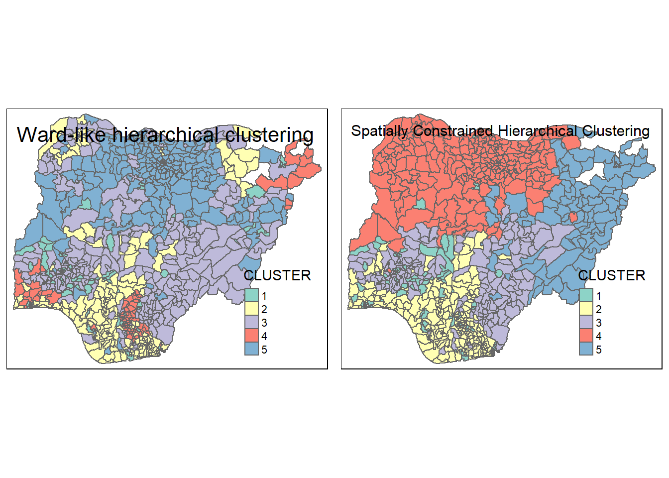
Visualisation on all clustering
The code chunk below is used to plot the clusters result together.
tmap_arrange(hclust.map, shclust.map, ngeoclust.map, gcluster.map, ncol = 2, asp = 1)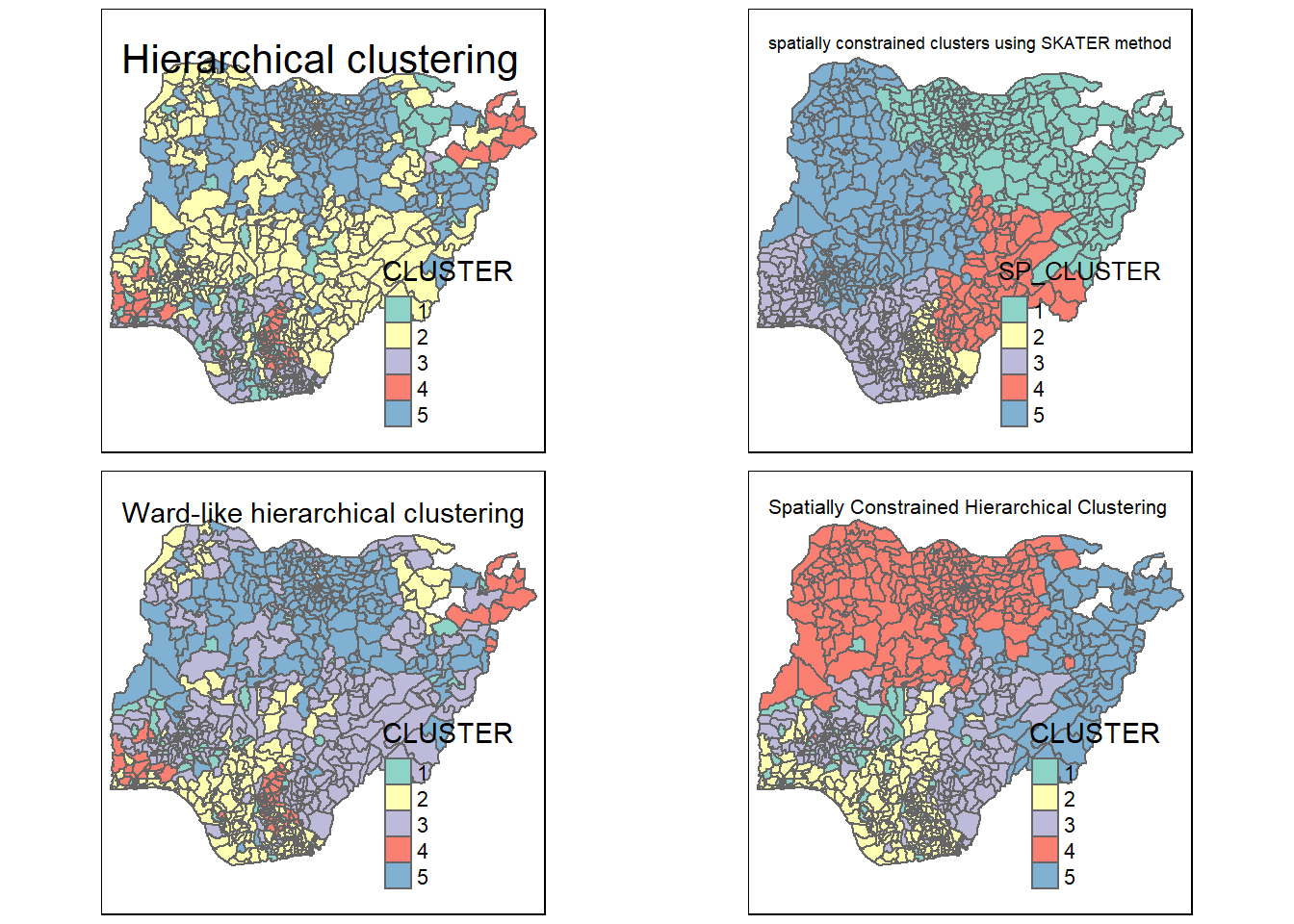
THE END.